Trapping capacities

Table 1 summarizes the theoretical trapping capacities for 23 of the formations found along the Norwegian Continental Shelf. These formation datasets were obtained from the NPD's CO₂ Storage Atlas [1]. Capacity calculations were done by using MRST-co2lab's trapAnalysis algorithm to determine the structural traps within the top surface, and using the formation properties summarized in Table 2. For details on how structural, residual, and dissolved trapping capacities are calculated, see Utsira's storage capacity estimate.

The estimates given for the North Sea formations can also been obtained using MRST-co2lab's interactive tool exploreCapacity, using the same input properties as given in Table 2. For example, when studying a formation found in the North Sea such as Utsira, set the water density to 1020 kg/m³ by the following:

     exploreCapacity('default_formation', 'Utsirafm',  'grid_coarsening', 1,  'water_density', 1020)

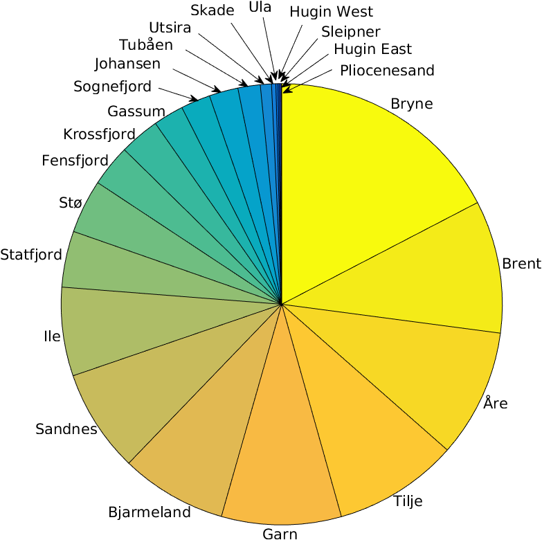
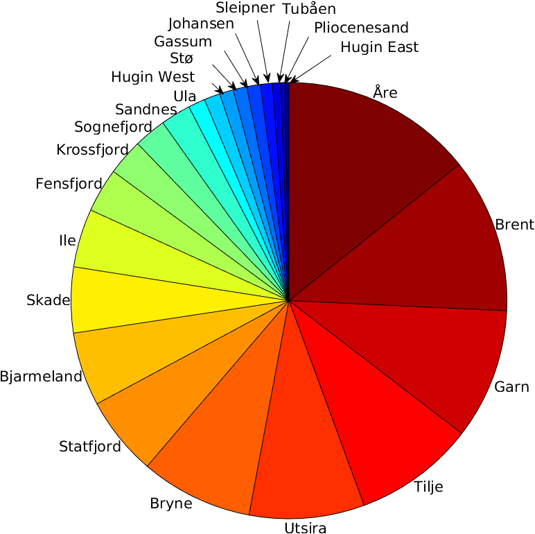
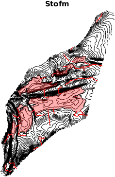
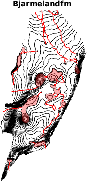
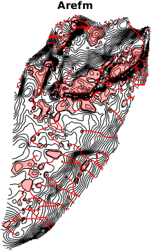
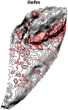
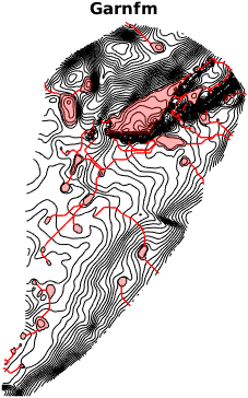
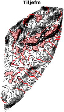
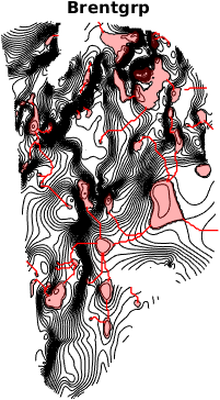
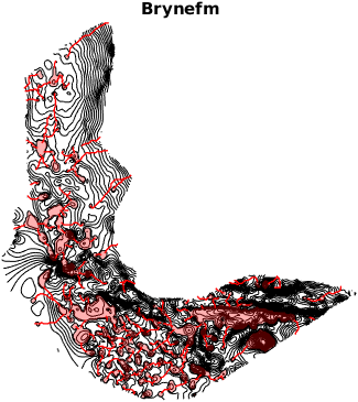
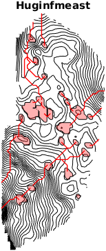
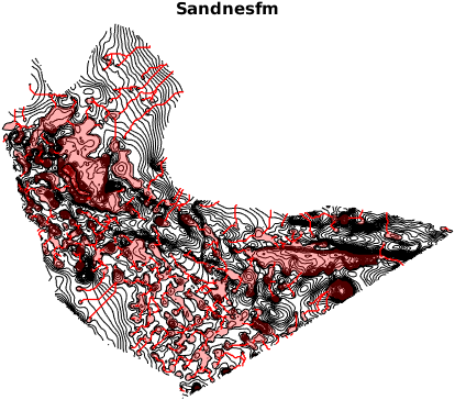
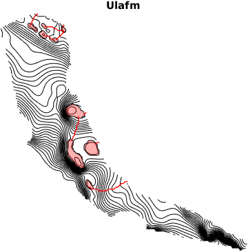
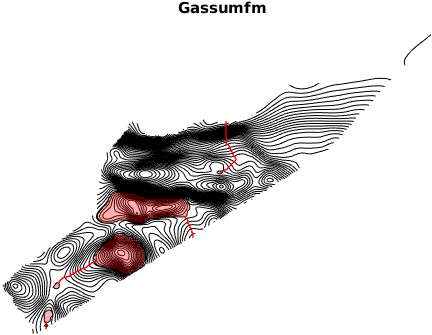
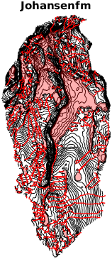
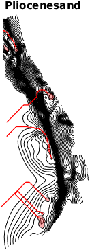
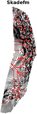
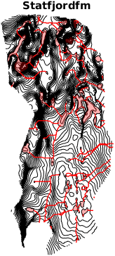
Click on the name of the formation in Table 1 to view a picture of the formation's top surface. In the picture, the black lines are the elevation contours of the top surface, regions colored in light red are the structural traps, and the red lines represent the rivers or spill-paths that connect individual structural traps along a spill-tree. More information about spill-point analysis including tutorials and examples can be found here.

Figure 1 illustrates that there is not necessarily a linear trend between structural trapping capacity and the total trapping capacity. For example, Utsira is ranked as the 5th highest in terms of total storage capacity (~118 Gt), however is the 7th lowest in terms of storage capacity in structural traps (~1 Gt). As another example, Bryne has the highest structural storage capacity (~24 Gt), but does not have the highest total storage capacity (rather ranked as the 6th highest in terms of total capacity (~114 Gt)).

Structural storage capacity (combined capacity = ~140 Gt)	Total storage capacity (combined capacity = ~1375 Gt)
Figure 1. Storage capacity comparison: in terms of structural trapping only (left) and in terms of all three trapping mechansims (right). Each wedge of the pie represents the amount that each formation contributes to the combined capacity of all 23 formations.

Theoretical versus practical storage capacity

The storage capacities presented here are the upper bounds of how much CO₂ could theoretically be stored in a given formation. These estimates assume that an entire formation can be utilized for storage, implying that CO₂ has filled the formation's pore volume. Such a scenario may be possible to achieve, however it may not be practical. For example, a large number of injection wells distributed over the formation could fill the entire formation pore volume with CO₂, however the cost associated with so many wells may be financially unfeasible. Other aspects that may make it impossible to utlize all of a formation's pore volume include CO₂ leakage through spill-paths, and the impact of pressure build-up on caprock integrity. Such aspects are related to the flow-dynamics, and are best investigated through simulation. Thus, in order to obtain practical storage capacities, it is nescessary to perform simulations of various injection scenarios for each formation.

References

1. E. K. Halland, J. Mujezinović, and F. Riis.CO₂ Storage Atlas: Norwegian Continental Shelf. Norwegian Petroleum Directorate, Stavanger, 2014.
2. V. Singh, A. Cavanagh, H. Hansen, B. Nazarian, M. Iding, and P. Ringrose. Reservoir Modeling of CO₂ Plume Behavior Calibrated Against Monitoring Data From Sleipner, Norway. In SPE Annual Technical Conference and Exhibition, Florence, Italy, 2010.
3. A. Chadwick, R. Arts, C. Bernstone, F. May, S. Thibeau, and P. Zweigel. Best Practice for the Storage of CO₂ in Saline Aquifers - Observations and Guidelines from the SACS and CO2STORE Projects. In British Geological Survey Occasional Publications, volume 14, pages 1-267. Nottingham, UK, 2008.
4. T. H. V. Pham, T. E. Maast, H. Hellevang, and P. Aagaard. Numerical Modeling including Hysteresis Properties for CO₂ Storage in Tubaen Formation, Snøhvit Field, Barents Sea. Energy Procedia, 4: 3746-3753, 2011.
5. E. Lundin, S. Polak, R. Bøe, P. Zweigel, and E. Lindberg. NGU Report 2005.027: Storage Potential for CO₂ in the Froan Basin Area of the Trøndelag Platform, Mid-Norway. Technical Report, Geological Survey of Norway / SINTEF, Trondheim, 2005.