Consider a two-phase oil-water problem. Solve the two-phase pressure equation

where v is the Darcy velocity (total velocity) and lambda is the mobility, which depends on the water saturation S.

The saturation equation (conservation of the water phase) is given as:

where phi is the rock porosity, f is the Buckley-Leverett fractional flow function, and q_w is the water source term.

We will use the corner-point geometry of a synthetic reservoir model from the SAIGUP study that has faults and inactive cells and hetereogeneous anisotropic permeability.

Contents

Decide which linear solver to use

We use MATLAB®'s built-in mldivide ("backslash") linear solver software to resolve all systems of linear equations that arise in the various discretzations. In many cases, a multigrid solver such as Notay's AGMG package may be prefereble. We refer the reader to Notay's home page at http://homepages.ulb.ac.be/~ynotay/AGMG/ for additional details on this package.

linsolve = @mldivide;

Check for existence of input model data

The model can be downloaded from the MRST page.

grdecl = fullfile(ROOTDIR, 'examples', 'data', 'saigup', 'SAIGUP.GRDECL');
if ~exist(grdecl, 'file'),
   error('Model data is not available.')
end

Read model data and convert units

The model data is provided as an ECLIPSE input file that can be read using the readGRDECL function.

grdecl = readGRDECL(grdecl);

MRST uses the strict SI conventions in all of its internal caluclations. The SAIGUP model, however, is provided using the ECLIPSE 'METRIC' conventions (permeabilities in mD and so on). We use the functions getUnitSystem and convertInputUnits to assist in converting the input data to MRST's internal unit conventions.

usys   = getUnitSystem('METRIC');
grdecl = convertInputUnits(grdecl, usys);

Define geometry and rock properties

We generate a space-filling geometry using the processGRDECL function and then compute a few geometric primitives (cell volumes, centroids, etc.) by means of the computeGeometry function.

G = processGRDECL  (grdecl);
G = computeGeometry(G);

The media (rock) properties can be extracted by means of the grdecl2Rock function.

rock = grdecl2Rock(grdecl, G.cells.indexMap);

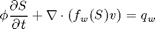
Modify the permeability to avoid singular tensors

The input data of the permeability in the SAIGUP realisation is an anisotropic tensor with zero vertical permeability in a number of cells. We work around this issue by (arbitrarily) assigning the minimum positive vertical (cross-layer) permeability to the grid blocks that have zero cross-layer permeability.

is_pos                = rock.perm(:, 3) > 0;
rock.perm(~is_pos, 3) = min(rock.perm(is_pos, 3));

Plot the logarithm of the permeability in the z-direction

clf,
   plotCellData(G,log10(rock.perm(:,3)),'EdgeColor','k','EdgeAlpha',0.1);
   axis off, view(-110,18); h=colorbar('horiz'); zoom(1.5)
   cs = [0.1 1 10 100 500 2000];
   caxis(log10([min(cs) max(cs)]*milli*darcy));
   set(h, 'XTick', log10(cs*milli*darcy), 'XTickLabel', num2str(round(cs)'));

Set fluid data

For the two-phase fluid model, we use values:

gravity off
fluid      = initSimpleFluid('mu' , [   1,   5]*centi*poise     , ...
                             'rho', [1000, 700]*kilogram/meter^3, ...
                             'n'  , [   2,   2]);

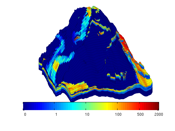
Introduce wells

The reservoir is produced using a set of production wells controlled by bottom-hole pressure and rate-controlled injectors. Wells are described using a Peacemann model, giving an extra set of equations that need to be assembled. For simplicity, all wells are assumed to be vertical and are assigned using the logical (i,j) subindex.

% Set vertical injectors, completed in the lowest 12 layers.
nz = G.cartDims(3);
I = [ 9,  8, 25, 25, 10];
J = [14, 35, 35, 95, 75];
R = [ 4,  4,  4,  4,  4,  4]*125*meter^3/day;
nIW = 1:numel(I); W = [];
for i = 1 : numel(I),
   W = verticalWell(W, G, rock, I(i), J(i), nz-11:nz, 'Type', 'rate', ...
                    'Val', R(i), 'Radius', 0.1, 'Comp_i', [1, 0], ...
                    'name', ['I$_{', int2str(i), '}$']);
end

% Set vertical producers, completed in the upper 14 layers
I = [17, 12, 25, 33, 7];
J = [23, 51, 51, 95, 94];
nPW = (1:numel(I))+max(nIW);
for i = 1 : numel(I),
   W = verticalWell(W, G, rock, I(i), J(i), 1:14, 'Type', 'bhp', ...
                    'Val', 300*barsa(), 'Radius', 0.1, ...
                    'name', ['P$_{', int2str(i), '}$'], 'Comp_i', [0, 1]);
end

% Plot grid outline and the wells
clf
   subplot('position',[0.02 0.02 0.96 0.96]);
   plotGrid(G,'FaceColor','none','EdgeAlpha',0.1);
   axis tight off, view(-120,50)
   plotWell(G,W,'height',200);
   plotGrid(G, vertcat(W(nIW).cells), 'FaceColor', 'b');
   plotGrid(G, vertcat(W(nPW).cells), 'FaceColor', 'r');

Initialize and construct the linear system

Initialize solution structures and assemble linear hybrid system from input grid, rock properties, and well structure.

S    = computeMimeticIP(G, rock, 'Verbose', true);
rSol = initState(G, W, 0, [0, 1]);

Using inner product: 'ip_simple'.
Computing cell inner products ...		Elapsed time is 9.530061 seconds.
Assembling global inner product matrix ...	Elapsed time is 0.087311 seconds.

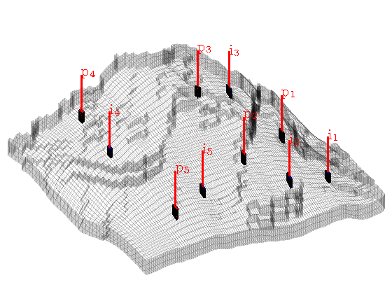
Solve initial pressure

Solve linear system construced from S and W to obtain solution for flow and pressure in the reservoir and the wells.

rSol = solveIncompFlow(rSol, G, S, fluid, 'wells', W, ...
                       'LinSolve', linsolve);
clf
   plotCellData(G, convertTo(rSol.pressure(1:G.cells.num), barsa), ...
                'EdgeColor', 'k', 'EdgeAlpha', 0.1);
   title('Initial pressure'), colorbar;
   plotWell(G, W, 'height', 200, 'color', 'k');
   axis tight off; view(-80,36); caxis([300 400])
   zoom(1.3)

Main loop

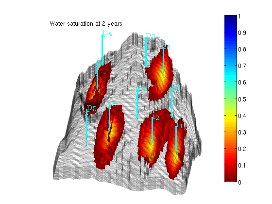
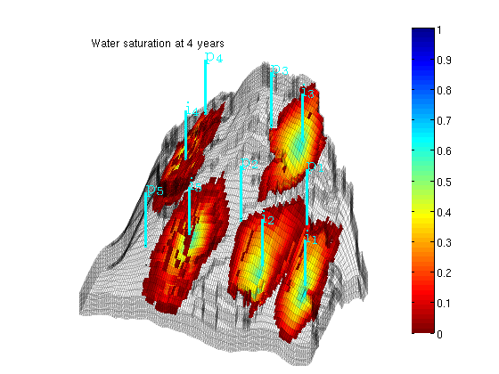
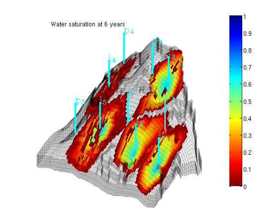
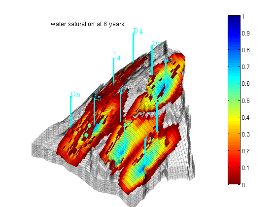
In the main loop, we alternate between solving the transport and the flow equations. The transport equation is solved using the standard implicit single-point upwind scheme with a simple Newton-Raphson nonlinear solver.

T      = 8*year();
dT     = T/4;
dTplot = 2*year();
pv     = poreVolume(G,rock);

% Prepare plotting of saturations
clf
   plotGrid(G, 'FaceColor', 'none', 'EdgeAlpha', 0.1);
   plotWell(G, W, 'height', 200, 'color', 'c');
   axis off, view(-80,30), colormap(flipud(jet))
   colorbar; hs = []; ha=[]; zoom(1.3);

% Start the main loop
t  = 0;  plotNo = 1;
while t < T,

   rSol = implicitTransport(rSol, G, dT, rock, fluid, 'wells', W);

   % Check for inconsistent saturations
   assert(max(rSol.s(:,1)) < 1+eps && min(rSol.s(:,1)) > -eps);

   % Update solution of pressure equation.
   rSol = solveIncompFlow(rSol, G, S, fluid, 'wells', W);

    % Increase time and continue if we do not want to plot saturations
   t = t + dT;
   if ( t < plotNo*dTplot && t continue, end

Plot saturation

   delete([hs, ha])
   hs = plotCellData(G, rSol.s(:,1), find(rSol.s(:,1) > 0.01));
   ha = annotation('textbox', [0.1714 0.8214 0.5000 0.1000], 'LineStyle', 'none', ...
                   'String', ['Water saturation at ', ...
                              num2str(convertTo(t,year)), ' years']);
   view(-80, 36), drawnow, caxis([0 1])
   plotNo = plotNo+1;

end

Published with MATLAB® 7.9