Example 5

This script contains MRST code necessary to produced the results discussed in Example 5. The basic setup is as in Figure 4 with a layered reservoir with lognormal permeability distribution, a vertical well in the center of the domain and Dirichlet boundary conditions at the left-hand side of the model.

Define the model
Visualize permeability
Partition the grid
Construct linear systems
Solve the global flow problems
Plot solution

Define the model

nx = 20; ny = 20; nz = 20;
Nx =  5; Ny =  5;
G         = cartGrid([nx ny nz]);
G         = computeGeometry(G);
[K, L]    = logNormLayers([nx, ny, nz], [200 45 350 25 150 300], 'sigma', 1);
rock.perm = convertFrom(K, milli*darcy);
fluid     = initSingleFluid('mu' ,    1*centi*poise     , ...
                            'rho', 1014*kilogram/meter^3);
gravity reset off

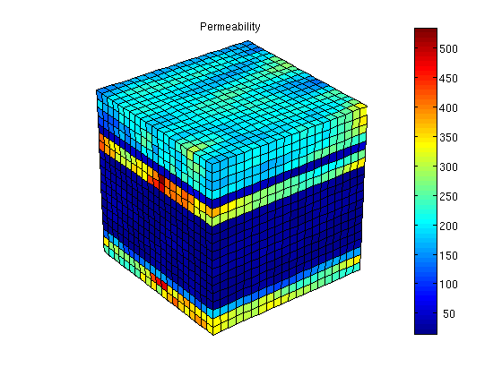
Visualize permeability

clf,
plotCellData(G,convertTo(rock.perm(:,1),milli*darcy)); shading faceted;
view(3), camproj perspective, axis tight equal off
h = colorbar('vert');
cs = 0:50:max(convertTo(rock.perm(:,1),milli*darcy));
set(h, 'YTick', cs, 'YTickLabel', num2str(cs'));
title('Permeability');

Model vertical well as a column of cell sources, each with rate equal 1 m^3/day. Set boundary conditions: a Dirichlet boundary condition of p=10 bar at the global left-hand side of the model

c   = (nx/2*ny+nx/2 : nx*ny : nx*ny*nz) .';
src = addSource([], c, ones(size(c)) ./ day());
bc = pside([], G, 'LEFT', 10*barsa());

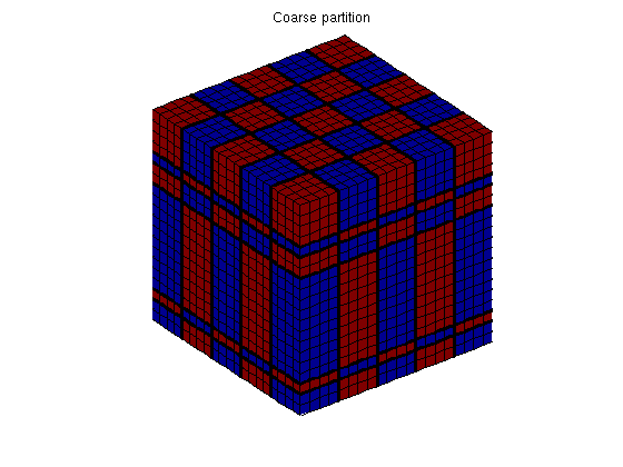
Partition the grid

We partition the fine grid into coarse blocks, ensuring that the coarse blocks do not cross the layers in our model (given by the vector L).

p = processPartition(G, partitionLayers(G, [Nx, Ny], L) );
clf,
plotCellData(G,mod(p,2)); shading faceted
outlineCoarseGrid(G,p,'LineWidth',3);
view(3); axis equal tight off, title('Coarse partition');

Construct linear systems

We build the grid structure for the coarse grid and construct the fine and the coarse system

CG = generateCoarseGrid(G, p);
S  = computeMimeticIP(G, rock);
CS = generateCoarseSystem(G, rock, S, CG, ones([G.cells.num, 1]), ...
                          'bc', bc, 'src', src);

Solve the global flow problems

xRef = solveIncompFlow  (initResSol(G, 0.0), G, S, fluid, ...
                         'src', src, 'bc', bc);
xMs  = solveIncompFlowMS(initResSol(G, 0.0), G, CG, p, S, CS, fluid,  ...
                         'src', src, 'bc', bc);

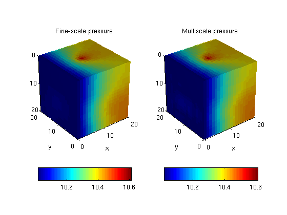
Plot solution

plot_pres = @(x) plotCellData(G,convertTo(x.pressure(1:G.cells.num), barsa()));
clf
subplot(1,2,1), cla
plot_pres(xRef);
view(3), camproj perspective, axis tight equal, camlight headlight
cax = caxis;  colorbar('location','southoutside'),title('Fine-scale pressure'), xlabel('x'), ylabel('y')

subplot(1,2,2), cla
plot_pres(xMs);
view(3), camproj perspective, axis tight equal, camlight headlight
caxis(cax); colorbar('location','southoutside'), title('Multiscale pressure'), xlabel('x'), ylabel('y')