Contents

A simple two phase problem solved using the Multiscale Finite Volume method

The multiscale finite volume method can easily be used in place of a regular pressure solver for incompressible transport. This example demonstrates a two phase solver on a 2D grid.

mrstModule add coarsegrid msfvm

Construct simple 2D Cartesian test case

nx = 50; ny = 50;
Nx = 5; Ny = 5;
G         = cartGrid([nx ny]);
G         = computeGeometry(G);

% Plot each timestep
doPlot = true;

p  = partitionUI(G, [Nx, Ny]);
CG = generateCoarseGrid(G, p);

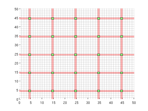
Generate dual grid

DG = partitionUIdual(CG, [Nx, Ny]);

Visualize

clf;
plotDual(G, DG)

Uniform permeability

rock.perm = repmat(100*milli*darcy, [G.cells.num, 1]);
rock.poro = repmat(0.3            , [G.cells.num, 1]);

T = computeTrans(G, rock);

Define a simple 2 phase fluid

fluid = initSimpleFluid('mu' , [   1,  10]*centi*poise     , ...
                            'rho', [1014, 859]*kilogram/meter^3, ...
                            'n'  , [   2,   2]);

Setup a producer / injector pair of wells

rate = 10*meter^3/day;
bhp  = 1*barsa;
radius = 0.05;
% Injector in lower left corner
W = addWell([], G, rock, round(nx/8) + nx*round(ny/8),      ...
            'Type', 'rate' , 'Val', rate, ...
            'Radius', radius, 'InnerProduct', 'ip_tpf', ...
            'Comp_i', [1, 0]);
% Producer in upper right corner
W = addWell(W, G, rock, round(7*nx/8) + nx*round(7*ny/8),      ...
            'Type', 'bhp' , 'Val', bhp, ...
            'Radius', radius, 'InnerProduct', 'ip_tpf', ...
            'Comp_i', [0, 1]);

Set up solution structures with only one phase

refSol    = initState(G, W, 0, [0, 1]);
msSol     = initState(G, W, 0, [0, 1]);

gravity off
verbose = false;

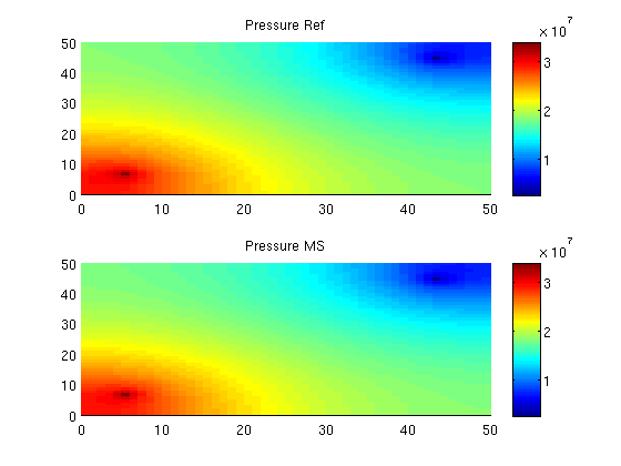
Set up pressure and transport solvers

We

% Reference TPFA
r_psolve = @(state) incompTPFA(state, G, T, fluid, 'wells', W);
% MsFV using a few iterations to improve flux error
psolve   = @(state) solveMSFV_TPFA_Incomp(state, G, CG, T, fluid, ...
                                                 'Reconstruct', true, 'Dual', DG, 'wells', W,...
                                                 'Update', true, 'Iterations', 5, 'Iterator', 'msfvm',...
                                                 'Subiterations', 10, 'Smoother', 'dms', 'Omega', 1);
% Implicit transport solver
tsolve   = @(state, dT) implicitTransport(state, G, dT, rock, ...
                                                fluid, 'wells', W, ...
                                                'verbose', verbose);

Alternatively we could have defined an explicit transport solver by

tsolve = @(state, dT, fluid) explicitTransport(state, G, dT, rock, fluid, ... 'wells', W, 'verbose', verbose);

Solve initial pressure in reservoir

We solve and plot the pressure in the reservoir at t=0.

refSol= r_psolve(refSol);
msSol = psolve(msSol);
subplot(2,1,1)
plotCellData(G, refSol.pressure); axis tight; colorbar;
title('Pressure Ref')
cbar = caxis();
subplot(2,1,2)
plotCellData(G, msSol.pressure); axis tight; colorbar;
title('Pressure MS')
caxis(cbar)

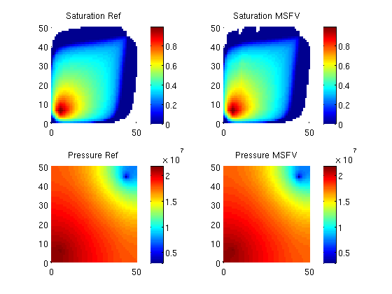
Transport loop

We solve the two-phase system using a sequential splitting in which the pressure and fluxes are computed by solving the flow equation and then held fixed as the saturation is advanced according to the transport equation.

T      = 20*day();
dT     = T/60;

Start the main loop

Iterate through the time steps and plot the saturation profiles along the way.

t = 0;
while t < T,
    % Solve transport equations using the transport solver
    msSol  = tsolve(msSol , dT);
    refSol = tsolve(refSol, dT);

    % Update the pressure based on the new saturations
    msSol    = psolve(msSol);
    refSol   = r_psolve(refSol);
    % Increase time and continue if we do not want to plot saturations
    if doPlot
        clf;
        % Saturation plot
        subplot(2,2,1)
        plotGrid(G, 'FaceColor', 'None', 'EdgeAlpha', 0)
        plotCellData(G, refSol.s(:,1), refSol.s(:,1) > 0); axis tight; colorbar;
        title('Saturation Ref')
        cbar = caxis();
        subplot(2,2,2)
        plotGrid(G, 'FaceColor', 'None', 'EdgeAlpha', 0)
        plotCellData(G, msSol.s(:,1), msSol.s(:,1) > 0); axis tight; colorbar;
        title('Saturation MSFV')
        % Align colorbars
        caxis(cbar)
        % Pressure plot
        subplot(2,2,3)
        plotCellData(G, refSol.pressure); axis tight; colorbar;
        title('Pressure Ref')
        cbar = caxis();
        subplot(2,2,4)
        hs = plotCellData(G, msSol.pressure); axis tight; colorbar;
        title('Pressure MSFV')
        caxis(cbar)
        drawnow
    end
    t = t + dT;
end