Contents

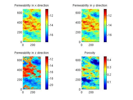
Document example dependcies

require impes spe10 deckformat

Define a oil/gas system

The fluid data is contained in the file 'simpleOilGas.txt'. We read and process this using the deckformat module.

current_dir = fileparts(mfilename('fullpath'));
f = fullfile(current_dir, 'simpleOilGas.txt');
deck = readEclipseDeck(f);

% Once the file has been read, we can use it to create the desired fluid.
fluid = initEclipseFluid(deck);

Set up grid and get petrophysical properties.

We select three layers to

layers = 25:28;
cartDims = [60, 220, numel(layers)];
physDims = cartDims.*[20,10,2]*ft;
rock = SPE10_rock(layers);
rock.perm = convertFrom(rock.perm, milli*darcy);

gravity off

% Define a Cartesian Grid based on the SPE layers selected.
G = cartGrid(cartDims, physDims);
G = computeGeometry(G);

% Cells with zero porosity are masked away to the minimum value to get
% sensible results.
is_pos = rock.poro>0;
rock.poro(~is_pos) = min(rock.poro(is_pos));

Show grid and petrophysical properties

Since the variations are large, use a logarithmic scale for permeability

perm = log10(rock.perm);
c = {'x', 'y', 'z'};
clf;
for i = 1:3
    subplot(2,2,i);
    plotCellData(G, perm(:,i));
    colorbar();
    axis equal tight;
    title(sprintf('Permeability in %s direction', c{i}));
end
% Plot porosity
subplot(2,2,4);
plotCellData(G, rock.poro);
colorbar();
axis equal tight;
title('Porosity')

Set up four producers at reservoir pressure and an injector at 500 bar

% Initialize empty well structure
W = [];

% Add an injector in the middle of the domain based on the midpoints of the
% cartesian indices
midpoint = round(cartDims)./2;

% Use vertical well, with completion in all layers. To complete in a
% different set of layers, enter the indices of the layers in completion
completion = [];
W = verticalWell(W, G, rock, midpoint(1), midpoint(2), completion, ...
                'Type', 'bhp',...            % Bottom hole pressure well
                'Val', 500*barsa,...         % Driving pressure
                'Radius', .125*meter, ...    % As per SPE10 Case B
                'InnerProduct', 'ip_tpf',... % Use TPFA inner product
                'Comp_i', [0, 1]);           % Injects only gas

% We want to place an producer in each corner of the domain, so we iterate
% over the corners and add a 200 bar well at each corner.
h_ind = [1, G.cartDims(1)];
v_ind = [1, G.cartDims(2)];
for i = 1:2
    for j = 1:2
        W = verticalWell(W, G, rock, h_ind(i), v_ind(j), [], ...
                        'Type', 'bhp',...
                        'Val', 200*barsa, ...
                        'Radius', .125*meter, ...
                        'InnerProduct', 'ip_tpf', ...
                        'Comp_i', [1, 0]);
    end
end

Compute one time values for the IMPES solver

Compute TPFA transmissibilities

Trans = computeTrans(G, rock);
% Compute pore volume
PV = poreVolume(G, rock);

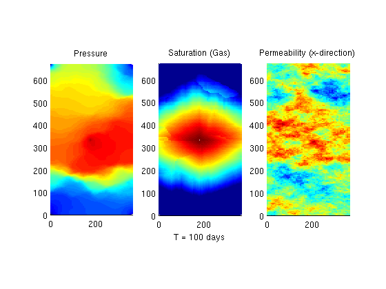
Initialize a oil filled reservoir at 200 bar.

Initially, it contains no gas

x = initResSolComp(G, W, fluid, 200*barsa, [1, 0]);

Do actual simulations

Simulate 100 days of production

dT = 1*day;
Nt = 100;

f1 = figure(1);
T  = 0;
tic()
for kk = 1:Nt,
   x = impesTPFA(x, G, Trans, fluid, dT, PV, 'wells', W);

    T = T + dT;

    % We skip drawing the values for the cells containing wells, since they
    % are always outliers.
    notPerf = ~ismember(1:G.cells.num, vertcat(W.cells));

    set(0, 'CurrentFigure', f1);
    clf;

    % Plot the pressure.
    subplot(1,3,1);
    plotCellData(G, (x.pressure), notPerf);
    title('Pressure')
    axis equal tight;

    % Plot the gas saturation
    subplot(1,3,2);
    plotCellData(G, log10(x.s(:,2)), notPerf);
    title('Saturation (Gas)')
    xlabel(sprintf('T = %1.0f days', convertTo(T, day)));
    axis equal tight;

    % Plot the x component of the permeability
    subplot(1,3,3);
    plotCellData(G, log10(rock.perm(:,1)));
    title('Permeability (x-direction)')
    axis equal tight;

    drawnow

end
toc()

Elapsed time is 168.679231 seconds.