You are here:
MRST
/
Modules
/
Deck Reader Module
/
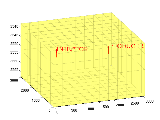
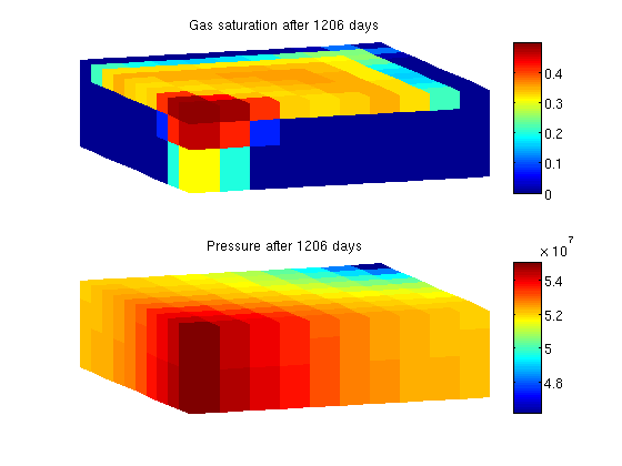
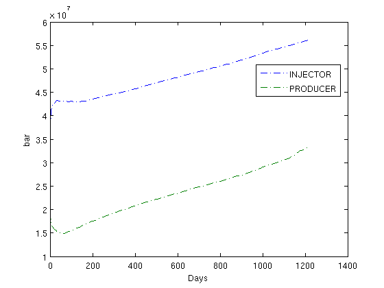
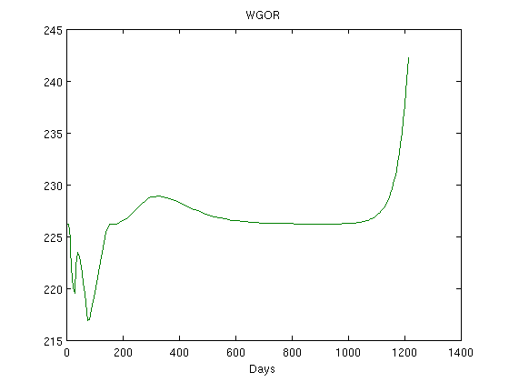
SPE1 Example