Example 6: Adaptive Refinement of Grid

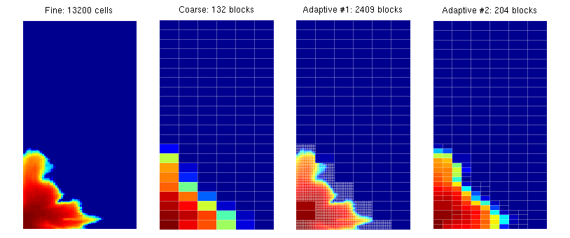
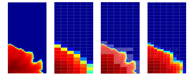
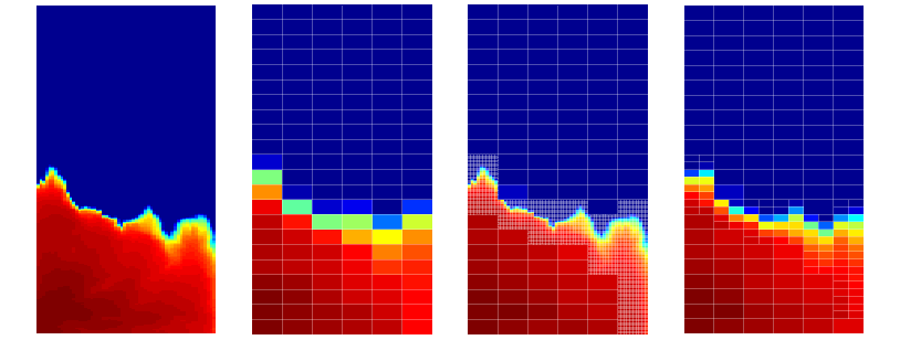
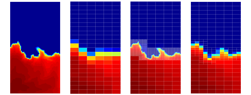
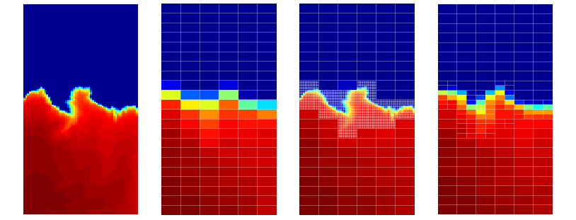
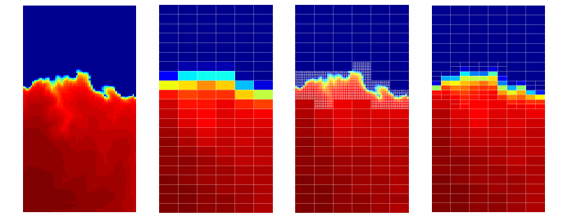
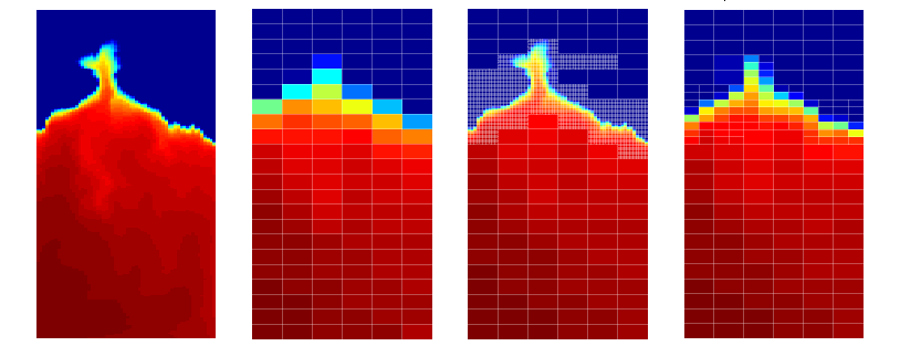
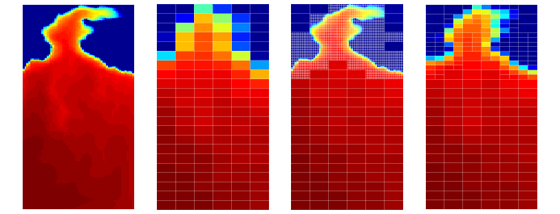
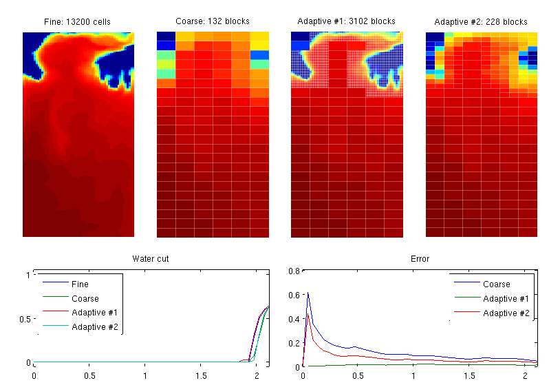
In this example, we show how to make grids that dynamically adapt to an advancing saturation front. To this end, we consider a quarter five-spot with heterogeneity sampled from on layer of the SPE10 data set. We will compare the solution transport on four different grids (using pressure solutions computed on the fine grid):

the original 60x220 fine grid
a coarse grid, which is either a Cartesian grid (if useCart=true) or a NUC grid based on the time-of-flight indicator and refineUniform
an adaptive grid with local refinement down to the original resolution
an adaptive grid with local refinement to intermediate resolution

Where to refine is predicted by comparing the solution at the previous time step with a coarse-grid estimation of the next time step. Refinement can then be imposed either cell-wise for all cells where the discrepancy is larger than satTol or blockwise in all blocks in which the discrepancy is larger than satTol. For the block-wise refinement, we also refine block neighbors across interfaces with net flux below fluxTol to reduce coarse-scale smearing.

References:

V. L. Hauge, K.-A. Lie, J. R. Natvig, Grid coarsening based on amalgamation for multi-fidelity transport solvers, September 2010, http://www.sintef.no/Projectweb/GeoScale/Publications/

Parameters controlling case setup
Initialize model problem and compute initial solution
Simulation parameters
Compute initial fine-grid solution
Create basic coarse grid and supporting data structures
Set correct fluxes for the state vectors
Time loop

Parameters controlling case setup

layer = 20;          % which layer from the SPE10 model
adaptBlocks = true;  % refine all cells within a marked block
useCart = true;      % use Cartesian coarse grid
satTol  = .02;       % refine if |s-s.old|>satTol
fluxTol = 1e-2;      % refine on both sides when net flux is below fluxTol

Initialize model problem and compute initial solution

Create grid structure, rock structure, and source structure, and initalise a fluid object. Note the viscosities. For simpler flow-pattern we use a quarter five-spot source/sink configuration, instead of the five-spot well configuration.

try
   require spe10
catch me
   mrstModule add spe10;
end
[G, W, rock] = SPE10_setup(25); clear W %#ok<ASGLU>
rock.poro    = max(rock.poro, 1e-3);
fluid        = initSimpleFluid('mu' , [   1,  .2]*centi*poise     , ...
                               'rho', [1014, 859]*kilogram/meter^3, ...
                               'n'  , [   2,   2]);
src  = addSource([], [1 G.cells.num], [1000 -1000]./day(), 'sat', [1, 0]);

Simulation parameters

param.nPres = 9;   % Pressure steps
param.nSub  = 5;   % Transport steps per pressure step
pv          = poreVolume(G, rock);
T           = .9 * sum(pv) / sum(src.rate(src.rate > 0)); % PVI -> time
DT          = T / (param.nPres * param.nSub);
[NL,NU]     = deal(50, 100);
[NLF,NUF]   = deal(10, 25);

Compute initial fine-grid solution

rf = initState(G, [], 0, 0);
S  = computeMimeticIP(G, rock);
rf = solveIncompFlow(rf, G, S, fluid, 'src', src);

Create basic coarse grid and supporting data structures

We generate a quite coarse grid used for estimatating which regions to refine adaptiv around the advancing saturation front. This is the same grid throughout the whole simulation process.

iTOF = log10(1 ./ ( ...
   computeTimeOfFlight(rf, G, rock, 'src', src) .* ...
   computeTimeOfFlight(rf, G, rock, 'src', src, 'reverse', true)));
iTOF  = iTOF - min(iTOF) + 1;

% Make static partitions and coarse grid
pS = partitionUI(G, [12 44 1]);
if useCart,
   p = partitionUI(G, [6 22 1]);
else
   p = segmentIndicator(G, iTOF, 2*round(max(iTOF) - min(iTOF)) ); %#ok<UNRCH>
   p = mergeBlocks2(p, G, pv, iTOF, NL, NU);
   p = refineBlocks(p, G, iTOF, NU, @refineGreedy2);
   p = mergeBlocks2(p, G, pv, iTOF, NL, NU);
   [b, bi, pS] = unique([pS, p], 'rows');
end
[blks, p] = findConfinedBlocks(G,p);
CG  = generateCoarseGrid(G, p);
pvC = accumarray(CG.partition,pv);

% Adding extra coarse grid fields to not stop in twophaseJacobian, getFlux
CG.cells.volumes = accumarray(CG.partition, G.cells.volumes);
CG.nodes.coords  = zeros(CG.cells.num, 3);
CG.faces.normals = zeros(CG.faces.num, 3);

% To find coarse net fluxes on coarse interfaces from fine fluxes
[nsubC, subC] = subFaces(G, CG);
[sgnC, cfC] = signOfFineFacesOnCoarseFaces(G, CG, nsubC, subC);

% Coarse rock and source structure
rockC.poro = accumarray(CG.partition, pv)./CG.cells.volumes;
srcC  = convertSource2Coarse(CG, src);

% Initially, all coarse grids are the same
aG1 = CG;
aG2 = CG;

Set correct fluxes for the state vectors

rf - fine grid rc - coarse grid, rc contains fine-grid and rcC coarse-grid quantities ra1 - adaptive #1, ra1 contains fine-grid and ra1C coarse-grid quantities ra2 - adaptive #2, ra2 contains fine-grid and ra2C coarse-grid quantities

rcC.flux       = accumarray(cfC, sgnC.*rf.flux(subC), [CG.faces.num,1]);
rcC.s          = coarse_sat(rf.s, CG.partition, pv, CG.cells.num);
[rc, ra1, ra2] = deal(rf);
[ra1C, ra2C]   = deal(rcC);
[ra1C.cflux, ra2C.cflux] = deal(rcC.flux);

Time loop

clf, set(gcf, 'OuterPosition', [444 454 820 640]);
wc  = zeros(param.nPres*param.nSub+1, 4); wc(2:end,:) = NaN;
err = zeros(param.nPres*param.nSub+1, 3); err(2:end,:) = NaN;
T   = 0:DT:T;
for i = 1:param.nPres,

   for j = 1:param.nSub,

      % Fine and coarse solution
      rf   = implicitTransport(rf, G, DT, rock, fluid, 'src', src);

      rcC  = implicitTransport(rcC, CG, DT, rockC, fluid, 'src', srcC);
      rc.s = rcC.s(CG.partition);

      % Adaptive grid with local fine-grid resolution
      % Predict new saturation on coarse grid
      est.flux = ra1C.cflux;
      est.s    = coarse_sat(ra1.s, CG.partition, pv, CG.cells.num);
      est      = implicitTransport(est, CG, DT, rockC, fluid, 'src', srcC);
      est.s    = est.s(CG.partition);

      % Determine which cells to refine
      if adaptBlocks,
         disc  = accumarray(CG.partition, abs(est.s - ra1.s).*pv)./ pvC;
         blks = [false; disc>satTol];
         N = double(CG.faces.neighbors( ...
            abs(ra1C.cflux) < fluxTol*max(ra1C.cflux),:)+1);
         blks(N(any(blks(N),2),:)) = true;
         blks = blks(2:end);
         cells = blks(CG.partition);
      else
         cells = abs(est.s - ra1.s)>satTol; %#ok<UNRCH>
      end

      % Update partition and create new grid
      pn        = CG.partition;
      pn(cells) = CG.cells.num + (1:sum(cells));
      pn        = compressPartition(pn);
      pn        = processPartition(G, pn);
      aG1       = generateCoarseGrid(G, pn);

       % Additional fields in the coarse grid
      aG1.cells.volumes = accumarray(aG1.partition, G.cells.volumes);
      aG1.nodes.coords  = zeros(aG1.cells.num, 3);
      aG1.faces.normals = zeros(aG1.faces.num, 3);

      % Updating structures
      [nsub,sub] = subFaces(G, aG1);
      [sgn,  cf] = signOfFineFacesOnCoarseFaces(G, aG1, nsub, sub);
      pvb        = accumarray(aG1.partition, pv);
      rockb.poro = pvb ./ aG1.cells.volumes;
      srcb       = convertSource2Coarse(aG1, src);
      ra1C.flux  = accumarray(cf, sgn .* ra1.flux(sub), [aG1.faces.num,1]);
      ra1C.s     = accumarray(aG1.partition, ra1.s.*pv) ./ pvb;

      % Transport simulation
      ra1C = implicitTransport(ra1C, aG1, DT, rockb, fluid, 'src', srcb);
      ra1.s = ra1C.s(aG1.partition);

      % Adaptive grid with local refinement (from pS)
      % Predict new saturation on coarse grid
      est.flux = ra2C.cflux;
      est.s    = coarse_sat(ra2.s, CG.partition, pv, CG.cells.num);
      est      = implicitTransport(est, CG, DT, rockC, fluid, 'src', srcC);
      est.s    = est.s(CG.partition);

      % Determine which cells to refine
      if adaptBlocks,
         disc  = accumarray(CG.partition, abs(est.s - ra2.s).*pv)./ pvC;
         blks = [false; disc>satTol];
         N = double(CG.faces.neighbors(...
            abs(ra2C.cflux) < fluxTol*max(ra2C.cflux),:)+1);
         blks(N(any(blks(N),2),:)) = true;
         blks = blks(2:end);
         cells = blks(CG.partition);
      else
         cells = abs(est.s - ra2.s)>satTol; %#ok<UNRCH>
      end

      % Update partition and create new coarse grid
      pn        = CG.partition;
      ps        = compressPartition(pS(cells));
      pn(cells) = max(pn) + ps;
      pn        = compressPartition(pn);
      pn        = processPartition(G, pn);
      aG2       = generateCoarseGrid(G, pn);

      % Additional fields in the coarse grid
      aG2.cells.volumes = accumarray(aG2.partition, G.cells.volumes);
      aG2.nodes.coords  = zeros(aG2.cells.num, 3);
      aG2.faces.normals = zeros(aG2.faces.num, 3);

      % Updating structures
      [nsub,sub] = subFaces(G, aG2);
      [sgn,  cf] = signOfFineFacesOnCoarseFaces(G, aG2, nsub, sub);
      pvb        = accumarray(aG2.partition, pv);
      rockb.poro = pvb ./ aG2.cells.volumes;
      srcb       = convertSource2Coarse(aG2, src);
      ra2C.flux  = accumarray(cf, sgn .* ra2.flux(sub), [aG2.faces.num,1]);
      ra2C.s     = accumarray(aG2.partition, ra2.s.*pv) ./ pvb;

      % Transport simulation on  aG2
      ra2C   = implicitTransport(ra2C, aG2, DT, rockb, fluid,  'src', srcb);
      ra2.s  = ra2C.s(aG2.partition);

      % Plotting of saturations
      clf
      axes('position',[.04 .35 .2 .6])
      plotCellData(G, rf.s), axis equal tight off
      title(sprintf('Fine: %d cells', G.cells.num));

      axes('position',[.28 .35 .2 .6])
      plotCellData(G, rc.s), axis equal tight off
      outlineCoarseGrid(G, CG.partition, 'EdgeColor', 'w', 'EdgeAlpha', 0.3);
      title(sprintf('Coarse: %d blocks', CG.cells.num));

      axes('position',[.52 .35 .2 .6])
      plotCellData(G, ra1.s), axis equal tight off
      outlineCoarseGrid(G, aG1.partition, 'EdgeColor', 'w', 'EdgeAlpha', 0.3);
      title(sprintf('Adaptive #1: %d blocks', aG1.cells.num))

      axes('position',[.76 .35 .2 .6])
      plotCellData(G, ra2.s), axis equal tight off
      outlineCoarseGrid(G, aG2.partition, 'EdgeColor', 'w', 'EdgeAlpha', 0.3);
      title(sprintf('Adaptive #2: %d blocks', aG2.cells.num));


      % Plot error curves and water cut
      ind = (i-1)*param.nSub + j+1;
      axes('position',[.06 .05 .42 .25])
      wc(ind,:) = [ rf.s(G.cells.num), rc.s(G.cells.num), ...
                    ra1.s(G.cells.num), ra2.s(G.cells.num) ];
      plot(T, wc),
      legend('Fine','Coarse', 'Adaptive #1', 'Adaptive #2', 2);
      axis([T(1) T(end) -.05 1.05]), title('Water cut')

      axes('position',[.54 .05 .42 .25])
      err(ind,:) = [sum(abs(rc.s - rf.s).*pv), ...
                    sum(abs(ra1.s - rf.s).*pv), ...
                    sum(abs(ra2.s - rf.s).*pv)]./sum(rf.s .* pv);
      plot(T, err),
      legend('Coarse', 'Adaptive #1', 'Adaptive #2', 1);
      set(gca,'XLim',[T(1) T(end)]), title('Error')

      drawnow
   end

   % Update fine-grid pressure
   rf  = solveIncompFlow(rf, G, S, fluid, 'src', src);

   % Update fine-grid pressure for CG, convert fluxes to coarse structure
   rc = solveIncompFlow(rc, G, S, fluid, 'src', src);
   rcC.flux = accumarray(cfC, sgnC .* rc.flux(subC), [CG.faces.num, 1]);

   % Update fine-grid pressure for aG1 and aG2
   ra1 = solveIncompFlow(ra1, G, S, fluid, 'src', src);
   ra2 = solveIncompFlow(ra2, G, S, fluid, 'src', src);

   % Compute net flux along underlying coarse grid
   ra1C.cflux = accumarray(cfC, sgnC .* ra1.flux(subC), [CG.faces.num, 1]);
   ra2C.cflux = accumarray(cfC, sgnC .* ra2.flux(subC), [CG.faces.num, 1]);
   % Fluxes for the adaptive coarse grid will be updated after the grid has
   % been generated in the main loop.