We present two examples of coarsening algorithms that fall into the general algorithmic framework described by Hauge et al [1]:

Both algorithms are applied to a 2D five-spot example with heterogeneity sampled from a lateral layer of the SPE10 model. For each algorithm, we consider three different flow indicators based on the absolute permeability, the velocity magnitude, and time-of-flight.

References:

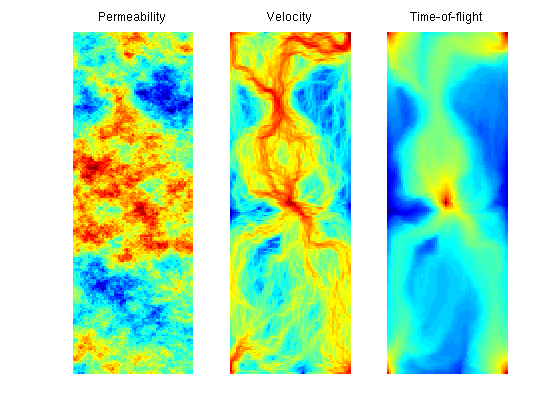
Contents

Set up and solve flow problem

As our example, we consider a standard five spot with heterogeneity sampled from Model 2 of the 10th SPE Comparative Solution Project.

try
   require spe10
catch me
   mrstModule add spe10;
end

try
   require gridtools
catch me
   mrstModule add gridtools;
end

[G, W, rock] = SPE10_setup(25);
rock.poro = max(rock.poro, 1e-4);
fluid = initSingleFluid('mu', 1*centi*poise, 'rho', 1014*kilogram/meter^3);
rS = initState(G, W, 0);
S  = computeMimeticIP(G, rock);
rS = solveIncompFlow(rS, G, S, fluid, 'wells', W);

We will use the following cell-wise indicators:

For all indicators, we perform a logarithmic scaling

clf
iK = log10(rock.perm(:,1)); iK = iK - min(iK) + 1;
subplot(1,3,1); plotCellData(G,iK); axis tight off
title('Permeability')

v  = faceFlux2cellVelocity(G, rS.flux); v  = sqrt(sum(v .^ 2, 2));
iV = log10(v); iV = iV - min(iV) + 1;
subplot(1,3,2); plotCellData(G,iV); axis tight off;
title('Velocity')

T  = computeTimeOfFlight(rS, G, rock, 'wells', W);
Tr = computeTimeOfFlight(rS, G, rock, 'wells', W, 'reverse', true);
iT = -log10(T.*Tr); iT = iT - min(iT) + 1;
subplot(1,3,3); plotCellData(G,iT); axis tight off;
title('Time-of-flight')

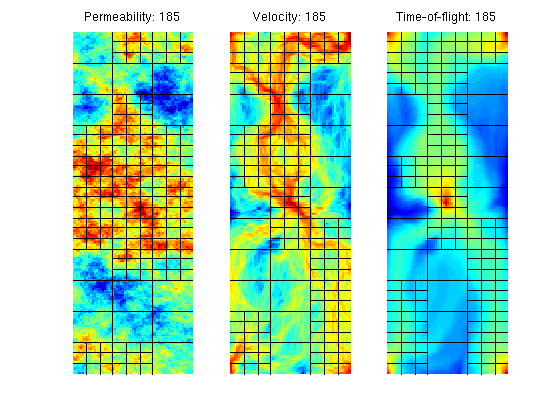
Uniform Refinement of High-Flow Zones

We start by a uniform 3x11 partition of the model and then add an extra 3x3 refinement in all blocks in which the block indicator exceeds the upper bound: Ib > NU*mean(Ic), where Ib is the indicator per block, Ic is the indicator per cell, and NU is a user-prescribed parameter.

p1 = partitionUI(G, [3, 11, 1]);
pK = refineBlocks(p1, G, iK, 380, @refineUniform, 'CartDims', [3,3,1]);
pV = refineBlocks(p1, G, iV, 390, @refineUniform, 'CartDims', [3,3,1]);
pT = refineBlocks(p1, G, iT, 380, @refineUniform, 'CartDims', [3,3,1]);

subplot(1,3,1)
outlineCoarseGrid(G, pK); title(sprintf('Permeability: %d', max(pK)))
subplot(1,3,2)
outlineCoarseGrid(G, pV); title(sprintf('Velocity: %d', max(pV)))
subplot(1,3,3)
outlineCoarseGrid(G, pT); title(sprintf('Time-of-flight: %d', max(pT)))

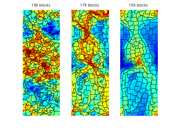
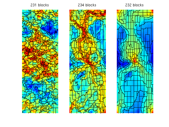
Using the two flow-based indicators iV and iT, rather than the a priori permeability indicator iK, gives grids that better adapt to the flow pattern. This is no surprise, since iK only distinguishes between zones with high permeability and low permeability, whereas the other two indicators also account for the influence of the forces that drive the flow.

The 'Nonuniform Coarsening' (NUC) Algorithm

Next, we consider the nonuniform coarsening algorithm and compare the grids generated using the three flow indicators introduced above

clf
numBins  = 10;
NL       = 30;
NU       = 80;

I = [iK iV iT];
for i=1:3
   p = segmentIndicator(G, I(:,i), numBins);
   p = mergeBlocks2(p, G, rock.poro, I(:,i), NL, NU);
   p = refineBlocks(p, G, I(:,i), NU, @refineGreedy2);
   p = mergeBlocks2(p, G, rock.poro, I(:,i), NL, NU);
   subplot(1,3,i), plotCellData(G, I(:,i)), outlineCoarseGrid(G,p);
   axis tight off, title(sprintf('%d blocks', max(p)));
end

Warning: Some blocks still violate lower (volume) bound after merging. 

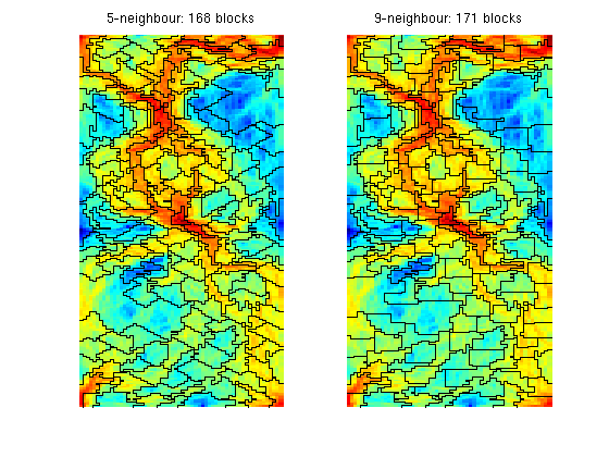
In the algorithm above, the greedy algorithm considers a 9-point neighbourhood when growing cells. In the original paper, the authors used a 5-point neighbourhood, which gives more diamond-shaped cells as shown in the figure below

clf
for i=1:2
   p = segmentIndicator(G, iV, numBins);
   p = mergeBlocks(p, G, rock.poro, iV, NL);
   p = refineBlocks(p, G, iV, NU, @refineGreedy2,'nlevel',i);
   p = mergeBlocks(p, G, rock.poro, iV, NL);
   subplot(1,2,i), plotCellData(G, iV), outlineCoarseGrid(G,p);
   axis tight off, title(sprintf('%d-neighbour: %d blocks', 2^(i+1)+1, max(p)));
end

In the two previous plots, we used the greedy algorithm to refine blocks. We can, of course, also other types of refinement algorithms of each block that exceeds the upper bound on the total flow. For a Cartesian grid, the 'refineUniform' method performs a uniform refinement of the bounding box of each block that exceeds the upper limit.

clf
for i=1:3
   p = segmentIndicator(G, I(:,i), numBins);
   p = mergeBlocks2(p, G, rock.poro, I(:,i), NL, NU);
   p = refineBlocks(p, G, I(:,i), NU, @refineUniform, 'CartDims',[2,2,1]);
   p = mergeBlocks2(p, G, rock.poro, I(:,i), NL, NU);
   subplot(1,3,i), plotCellData(G, I(:,i)), outlineCoarseGrid(G,p);
   axis tight off, title(sprintf('%d blocks', max(p)));
end

Warning: Some blocks still violate lower (volume) bound after merging.