SPE9

Ninth Comparative Solution Project
Set up model
Set up linear solver
Plot the rock permeability
Plot the grid porosity
Plot a single vertical set of cells
Plot initial saturation of oil and water
Examine gas dissolved in oil phase
Plot the wells
Examine the schedule
Examine well limits
Plot relative permeability curves
Plot three-phase relative permeability
Plot capillary pressure curves
Plot compressibility
Plot oil compressibility
Plot the viscosity
Simulate the schedule
Launch interactive plot tool for well curves
Load comparison data from commercial solver
Set up plotting functions
Plot two different producers
Plot the gas production rate
Changing controls
Plot pressure before and after schedule
Plot free gas
Plot dissolved gas
Plot phase distribution
Copyright notice

Ninth Comparative Solution Project

This example runs the model from the SPE9 benchmark, which was posed twenty years ago to compare contemporary black-oil simulators (Killough, 1995). The reservoir is described by a 24 x 25 x 15 grid, having a 10 degree dipping-angle in the x-direction. By current standards, the model is quite small, but contains a few features that will still pose challenges for black-oil simulators. The 25 producers initially operate at a maximum rate of 1500 STBO/D, which is lowered to 100 STBO/D from day 300 to 360, and the raised up again to its initial value until the end of simulation at 900 days. The single water injector is set to a maximum rate of 5000 STBW/D with a maximum bottom-hole pressure of 4000 psi at reference depth. This setup will cause free gas to form after ~100 days when the reservoir pressure is reduced below the original saturation pressure. The free gas migrates to the top of the reservoir. During the simulation most of the wells convert from rate control to pressure control. A second problem is a discontinuity in the water-oil capillary pressure curve, which may cause difficulties in the Newton solver when saturations are changing significantly.

In this comprehensive example, we will discuss the various parameters that enter the model and show how to set up state-of-the-art simulation using a CPR preconditioner with algebraic multigrid solver.

Killough, J. E. 1995. Ninth SPE comparative solution project: A reexamination of black-oil simulation. In SPE Reservoir Simulation Symposium, 12-15 February 1995, San Antonio, Texas. SPE 29110-MS, doi: 10.2118/29110-MS

mrstModule add ad-blackoil ad-core mrst-gui ad-props deckformat

Set up model

This SPE comparative solutions project problem consists of a water injection problem in a highly heterogenous reservoir. There is one injector and 25 producers. The problem is set up to be solved using a black-oil model. The data set we provide is a modified version of input files belonging to the course in reservoir engineering and petrophysics at NTNU (Trondheim, Norway) and available at http://www.ipt.ntnu.no/~kleppe/pub/SPE-COMPARATIVE/ECLIPSE_DATA/.

We have put most of the boilerplate setup into the setupSPE9 function.

[G, rock, fluid, deck, state0] = setupSPE9();

% Determine the model automatically from the deck. It should be a
% three-phase black oil model with gas dissoluton.
model = selectModelFromDeck(G, rock, fluid, deck);
% Set maximum limits on saturation, Rs and pressure changes
model.drsMaxRel = .2;
model.dpMaxRel  = .2;
model.dsMaxAbs  = .05;

% Show the model
model %#ok, intentional display

% Convert the deck schedule into a MRST schedule by parsing the wells
schedule = convertDeckScheduleToMRST(model, deck);

model = 
  ThreePhaseBlackOilModel with properties:

                     disgas: 1
                     vapoil: 0
                  drsMaxRel: 0.2000
                  drsMaxAbs: Inf
                      fluid: [1x1 struct]
                       rock: [1x1 struct]
                   dpMaxRel: 0.2000
                   dpMaxAbs: Inf
                   dsMaxRel: Inf
                   dsMaxAbs: 0.0500
            maximumPressure: Inf
            minimumPressure: -Inf
                      water: 1
                        gas: 1
                        oil: 1
         saturationVarNames: {'sw'  'so'  'sg'}
          componentVarNames: {}
               wellVarNames: {'qWs'  'qOs'  'qGs'  'bhp'}
          useCNVConvergence: 1
               toleranceCNV: 1.0000e-03
                toleranceMB: 1.0000e-07
           toleranceWellBHP: 100000
          toleranceWellRate: 1.1574e-05
                  inputdata: [1x1 struct]
           extraStateOutput: 0
         extraWellSolOutput: 1
               outputFluxes: 1
    upstreamWeightInjectors: 0
                    gravity: [0 0 9.8066]
                  wellmodel: [1x1 WellModel]
                  operators: [1x1 struct]
         nonlinearTolerance: 1.0000e-06
                          G: [1x1 struct]
                    verbose: 0
       stepFunctionIsLinear: 0

Set up linear solver

We proceed to setup a CPR-type solver, using the AGMG linear solver as the multigrid preconditioner. The CPR preconditioner attempts to decouple the fully implicit equation set into a pressure component and a transport component.

The pressure is mathematically elliptic/parabolic in nature, and multigrid is well suited for solving these highly coupled, challenging problems. The remainder of the linear system, corresponding to the hyperbolic part of the equations is localized in nature and is primarily concerned with moving the saturation between neighboring grid blocks.

Setting up a preconditioner is not strictly required to solve this problem, as the 9000 cells for a three-phase system results in linear systems with 27000 unknowns (one equation per phase, per cell). However, it does improve the solution speed and is required for larger cases, where Matlab's standard linear solvers scale poorly.

try
    mrstModule add agmg
    pressureSolver = AGMGSolverAD('tolerance', 1e-4);
catch
    pressureSolver = BackslashSolverAD();
end
linsolve = CPRSolverAD('ellipticSolver', pressureSolver);

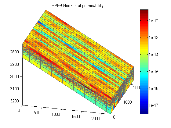
Plot the rock permeability

The SPE9 data set has an anisotropic, inhomogenous permeability field. The vertical permeability is 1/10th of the horizontal values. We plot the permeability using a log10 transform to better see the contrast.

v = [15, 30];
[G, rock] = deal(model.G, model.rock);

clf
plotCellData(G, log10(rock.perm(:, 1)))
logColorbar(); axis tight, view(v)
title('SPE9 Horizontal permeability');

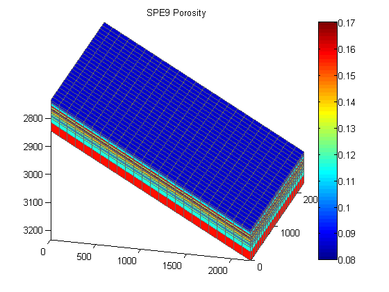
Plot the grid porosity

cla
plotCellData(G, rock.poro)
colorbar()
title('SPE9 Porosity');

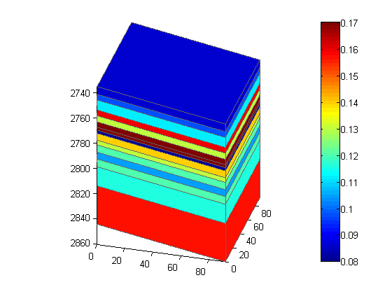
Plot a single vertical set of cells

While the grid is structured, the grid has varying cell size along the vertical axis. To show this in detail, we plot the porosity in a single column of cells. We get the underlying logical grid and extract the subset corresponding to the first column (upper left corner of the grid).

By using axis equal we see the actual aspect ratio of the cells.

clf
[ii, jj] = gridLogicalIndices(G);
plotCellData(G, rock.poro, ii == 1 & jj == 1)
colorbar, axis equal tight, view(v)

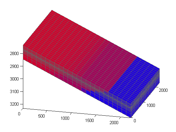
Plot initial saturation of oil and water

Initially, the reservoir does not contain free gas. We plot the initial saturations using the RGB plotting feature, where a three column matrix sent to plotCellData is interpreted column wise as fractions of red, green and blue respectively. Since MRST convention is to order the phases in the order WOG we need to permute the column index slightly to get red oil, blue water and green gas.

s = state0.s(:, [2, 3, 1]);
clf
plotCellData(G, s)
axis tight; view(v)

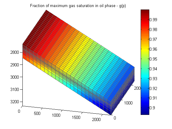
Examine gas dissolved in oil phase

Even though there is no free gas initially, there is significant amounts of gas dissolved in the oil phase. The dissolved gas will bubble into free gas when the pressure drops below the bubble point pressure. For a given pressure there is a fixed amount of gas that can be dissolved in the black-oil instantanous dissolution model. To illustrate how saturated the initial conditions are, we plot the function

I.e. how close the oil phase is to being completely saturated for the current pressure. A value near one means that the liquid is close to saturated and any values above one will immediately lead to free gas appearing in the simulation model.

As we can see from the figure, free gas will appear very quickly should the pressure drop.

Rs_sat = model.fluid.rsSat(state0.pressure);
Rs = state0.rs;

clf
plotCellData(G, Rs./Rs_sat)
axis tight; colorbar, view(v)
title('Fraction of maximum gas saturation in oil phase - g(p)');

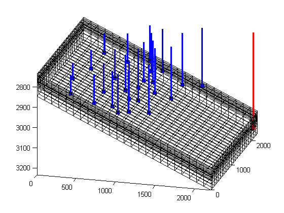
Plot the wells

Since there is a large number of wells, we plot the wells without any labels and simply color the injector in blue and the producers in red.

W = schedule.control(1).W;
sgn = [W.sign];
clf
plotGrid(G, 'FaceColor', 'none')
plotWell(G, W(sgn>0), 'fontsize', 0, 'color', 'b')
plotWell(G, W(sgn<0), 'fontsize', 0, 'color', 'r')
axis tight; view(v)

Examine the schedule

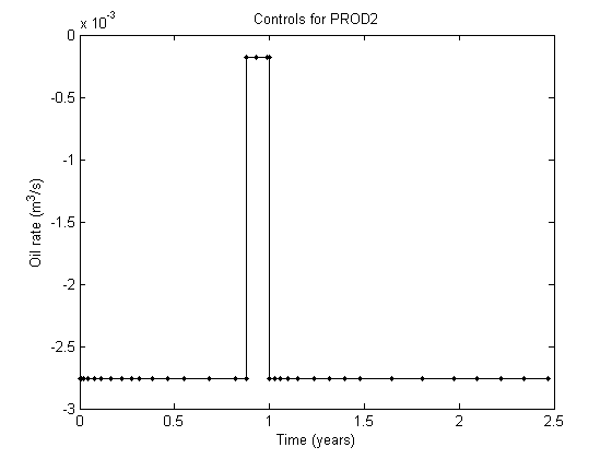
The simulation schedule consists of three control periods. All 26 wells are present during the entire simulation, but their prescribed rates will change. The injector is injecting a constant water rate, while the producers all produce a constant oil rate, letting bottom hole pressures and gas/water production vary. Since all producers have the same controls, we can examine PROD2 in detail. We plot the controls, showing that the well rate drops sharply midway during the simulation

wno = find(strcmp({schedule.control(1).W.name}, 'PROD2'));

% Extract controls for all timesteps
P = arrayfun(@(ctrl) schedule.control(ctrl).W(wno).val, schedule.step.control);
T = cumsum(schedule.step.val);
stairs(T/year, P, '.-k')
xlabel('Time (years)')
ylabel('Oil rate (m^3/s)')
title('Controls for PROD2')

Examine well limits

Note that the well controls are not the only way of controlling a well. Limits can be imposed on wells, either due to physical or mathematical considerations. In this case, fixed oil rate is the default setting, but the well will switch controls if the pressure drops below a threshold. This is found in the lims field for each well.

Since this is a producer, the bhp limit is considered a lower limit, whereas a bhp limit for an injector would be interpreted as a maximum limit to avoid either equipment failure or formation of rock fractures.

clc
disp(['Well limits for ', schedule.control(1).W(wno).name, ':'])
disp(schedule.control(1).W(wno).lims)

Well limits for PROD2:
    orat: -0.0028
    wrat: -Inf
    grat: -Inf
    lrat: -Inf
     bhp: 6.8948e+06

Plot relative permeability curves

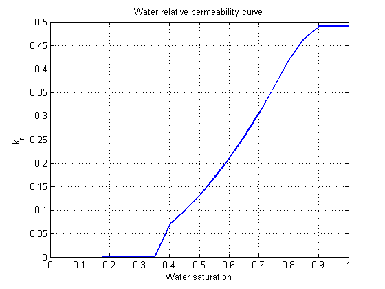
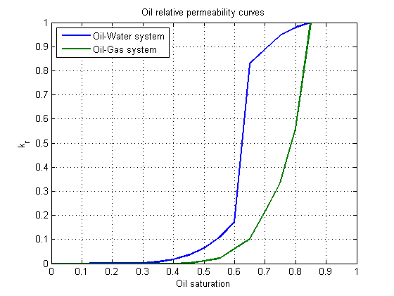
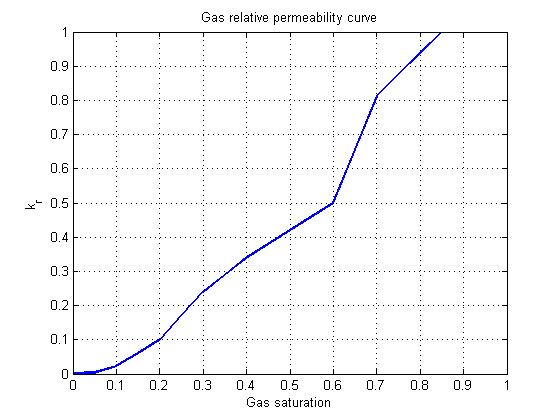
For a three-phase model we have four relative permeability curves. One for both gas and water and two curves for the oil phase. The oil relative permeability is tabulated for both water-oil and oil-gas systems, and as we can see from the following plot, this gives a number of kinks that will tend to pose challenges for the Newton solver.

f = model.fluid;
s = (0:0.05:1)';

figure;
plot(s, f.krW(s), 'linewidth', 2)
grid on
xlabel('Water saturation');
title('Water relative permeability curve')
ylabel('k_r')

figure;
plot(s, [f.krOW(s), f.krOG(s)], 'linewidth', 2)
grid on
xlabel('Oil saturation');
legend('Oil-Water system', 'Oil-Gas system', 'location', 'northwest')
title('Oil relative permeability curves')
ylabel('k_r')

figure;
plot(s, f.krG(s), 'linewidth', 2)
grid on
xlabel('Gas saturation');
title('Gas relative permeability curve')
ylabel('k_r')

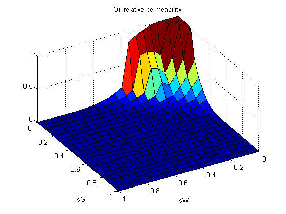
Plot three-phase relative permeability

When all three phases are present simultaneously in a single cell, we need to use some functional relationship to combine the two-phase curves in a reasonable manner, resulting in a two-dimensional relative permeability model. Herein, we use the Stone I model.

close all

[x, y] = meshgrid(s);
krO = zeros(size(x));

for i = 1:size(x, 1)
    xi = x(i, :);
    yi = y(i, :);
    [~, krO(i, :), ~] = model.relPermWOG(xi, 1 - xi - yi, yi, f);
end
figure;
surf(x, y, krO)
xlabel('sW')
ylabel('sG')
title('Oil relative permeability')
view(150, 50); axis tight

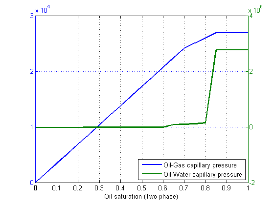
Plot capillary pressure curves

SPE9 contains significant capillary pressure, making the problem more nonlinear as the flow directions and phase potential gradients are highly saturation dependent. Again we have two curves, one for the contact between oil and gas and another for the water-oil contact.

close all
figure;
[ax, l1, l2] = plotyy(s, f.pcOG(s), s, f.pcOW(1 - s));
set([l1, l2], 'LineWidth', 2);
grid on
legend('Oil-Gas capillary pressure', 'Oil-Water capillary pressure', 'location', 'southeast')
xlabel('Oil saturation (Two phase)')

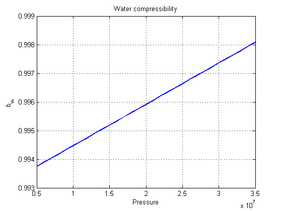
Plot compressibility

The black-oil model treats fluid compressibility through tabulated functions often referred to as formation volume factors (or B-factors). To find the mass of a given volume at a specific reservoir pressure , we write

where refers to either the phase, V_R the volume occupied at reservoir conditions and is the surface / reference density when the B-factor is 1.

Note that MRST by convention only uses small b to describe fluid models. The relation between B and b is simply the reciprocal and will be calculated when needed.

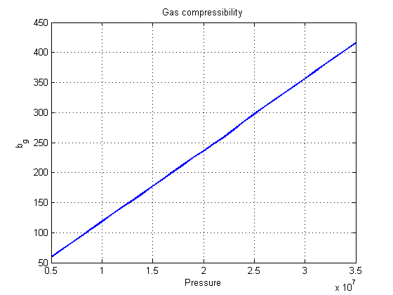
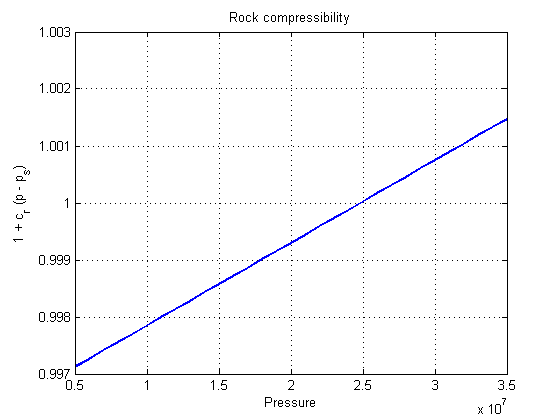
We begin by plotting the B-factors/compressibility for the water and gas phases. Note that the water compressibility is minimal, as water is close to incompressible in most models. The gas compressibility varies several orders of magnitude.

The rock compressibility is included as well. Rock compressibility is modelling the poroelastic expansion of the pore volume available for flow. As the rock itself shrinks, more fluid can fit inside it.

Note that although the curves shown in this particular case are all approximately linear, there is no such requirement on the fluid model.

pressure = (50:10:500)'*barsa;

close all
figure;
plot(pressure/barsa, 1./f.bW(pressure), 'LineWidth', 2);
grid on
title('Water formation volume factor')
ylabel('B_w')
xlabel('Pressure [bar]');

figure;
plot(pressure/barsa, 1./f.bG(pressure), 'LineWidth', 2);
grid on
title('Gas formation volume factor')
ylabel('B_g')
xlabel('Pressure [bar]');

figure;
plot(pressure/barsa, f.pvMultR(pressure), 'LineWidth', 2);
grid on
title('Rock compressibility')
ylabel('1 + c_r (p - p_s)')
xlabel('Pressure [bar]');

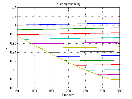
Plot oil compressibility

Since we allow the gas phase to dissolve into the oil phase, compressibility does not only depend on the pressure: The amount of dissolved gas will also change how much the fluid can be compressed.

We handle this by having saturated and undersatured tables for the formation volume factors (FVF). This is reflected in the figure: Unsaturated FVF curves will diverge into from the main downwards sloping trend into almost constant curves sloping downwards.

Physically, the undersaturated oil will swell as more gas is being introduced into the oil, increasing the volume more than the pressure decreases the volume of the oil itself. When the oil is completely saturated, the volume decrease is due to the gas-oil mixture itself being compressed.

rs = 0:25:320;
[p_g, rs_g] = meshgrid(pressure, rs);
rssat = zeros(size(p_g));
for i = 1:size(p_g, 1)
    rssat(i, :) = f.rsSat(p_g(i, :));
end

saturated = rs_g >= rssat;
rs_g0 = rs_g;
rs_g(saturated) = rssat(saturated);

figure;
plot(p_g'/barsa, 1./f.bO(p_g, rs_g, saturated)', 'LineWidth', 2)
grid on
title('Oil formation volume factor')
ylabel('B_o')
xlabel('Pressure [bar]')

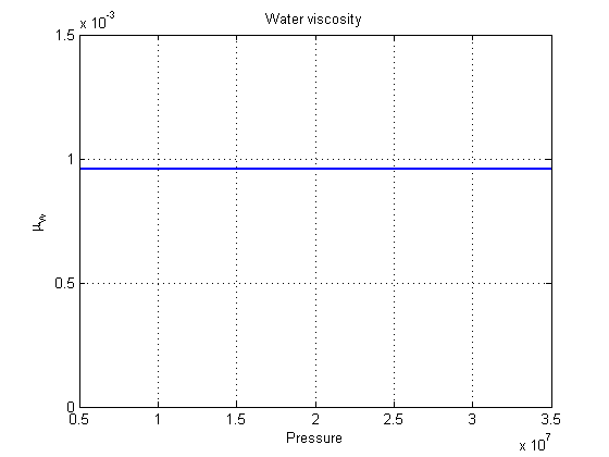
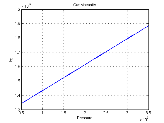
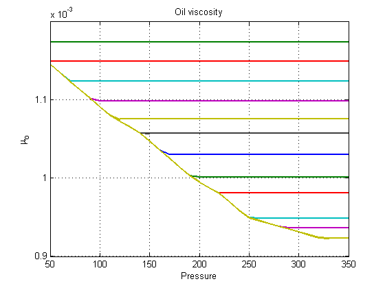
Plot the viscosity

The viscosity can also depend on the pressure and dissolved components in a similar manner as the compressibility. Again, we note that the water phase is unaffected by the pressure, the gas changes viscosity quite a bit. As with , the oil viscosibility depends more on the amount of dissolved gas than the pressure itself and we have undersatured tables to show.

SPE9 only allows gas to dissolve into oil, and not the other way around. Generally, the black-oil model is a pseudo-compositional model where both gas in oil () and oil in gas () can be included.

close all
figure;
plot(pressure, f.muW(pressure), 'LineWidth', 2);
grid on
title('Water viscosity')
ylabel('\mu_w')
xlabel('Pressure');
ylim([0, 1.5e-3])

figure;
plot(pressure, f.muG(pressure), 'LineWidth', 2);
grid on
title('Gas viscosity')
ylabel('\mu_g')
xlabel('Pressure');

figure;
plot(p_g'/barsa, f.muO(p_g, rs_g, saturated)', 'LineWidth', 2)
grid on
title('Oil viscosity')
ylabel('\mu_o')
xlabel('Pressure')

Simulate the schedule

We run the schedule. We provide the initial state, the model (containing the black oil model in this case) and the schedule with well controls, and control time steps. The simulator may use other timesteps internally, but it will always return values at the specified control steps.

close all
model.verbose = false;
fn = getPlotAfterStep(state0, model, schedule, ...
    'plotWell', false, 'plotReservoir', false);
[wellsols, states, reports] =...
    simulateScheduleAD(state0, model, schedule, ...
                       'LinearSolver', linsolve, 'afterStepFn', fn);

Solving timestep 01/35:                   -> 1 Day
Well INJE1: Control mode changed from rate to bhp.
Well PROD26: Control mode changed from orat to bhp.
Solving timestep 02/35: 1 Day             -> 2 Days
...
Well PROD24: Control mode changed from orat to bhp.
Solving timestep 35/35: 2 Years, 125 Days -> 2 Years, 170 Days
*** Simulation complete. Solved 35 control steps in 307 Seconds, 924 Milliseconds ***

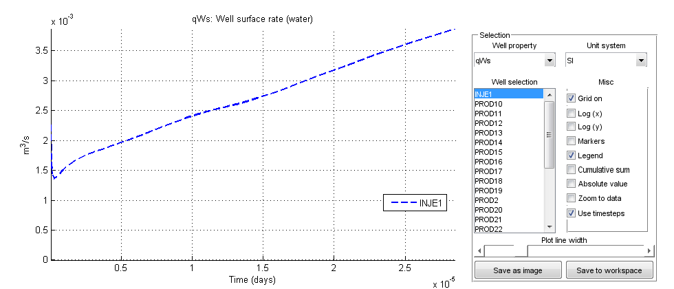
Launch interactive plot tool for well curves

The interactive viewer can be used to visualize the wells and is the best choice for interactive viewing.

plotWellSols(wellsols, cumsum(schedule.step.val), 'field', 'qTr')
h = gcf;

Load comparison data from commercial solver

To validate the simulator output, we load in a pre-run dataset from a industry standard commercial solver run using the same inputs.

addir = mrstPath('ad-blackoil');
compare = fullfile(addir, 'examples', 'spe9', 'compare');
smry = readEclipseSummaryUnFmt(fullfile(compare, 'SPE9'));

compd = 1:(size(smry.data, 2));
Tcomp =  smry.get(':+:+:+:+', 'YEARS', compd);

Set up plotting functions

We will plot the timesteps with different colors to see the difference between the results clearly.

if ishandle(h);
    close(h);
end
T = convertTo(cumsum(schedule.step.val), year);

mrstplot = @(data) plot(T, data, '-b', 'linewidth', 2);
compplot = @(data) plot(Tcomp, data, 'ro', 'linewidth', 2);

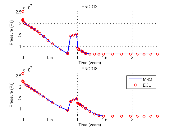
Plot two different producers

We plot the bottom-hole pressures for two somewhat arbitrarily chosen producers to show the accuracy of the pressure.

clf
names = {'PROD13', 'PROD18'};
nn = numel(names);
for i = 1:nn

    name = names{i};

    comp = convertFrom(smry.get(name, 'WBHP', compd), psia)';
    mrst = getWellOutput(wellsols, 'bhp', name);

    subplot(nn, 1, i)
    hold on
    mrstplot(mrst);
    compplot(comp);
    title(name)
    axis tight
    grid on

    xlabel('Time (years)')
    ylabel('Pressure (Pa)')
end
legend({'MRST', 'ECL'})

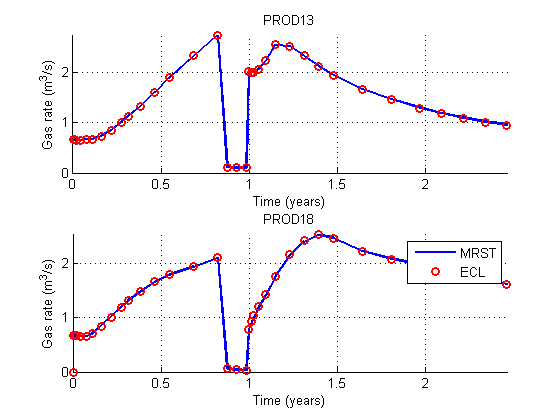
Plot the gas production rate

We plot the gas production rate (at surface conditions).

clf
for i = 1:nn
    name = names{i};
    comp = convertFrom(smry.get(name, 'WGPR', compd), 1000*ft^3/day);
    mrst = abs(getWellOutput(wellsols, 'qGs', name));

    subplot(nn, 1, i)
    hold on
    mrstplot(mrst);
    compplot(comp);
    title(name)
    axis tight
    grid on

    xlabel('Time (years)')
    ylabel('Gas rate (m^3/s)')
end
legend({'MRST', 'ECL'})

Changing controls

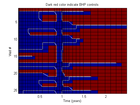
We saw earlier that all wells are initially rate controlled, but in practice a large number of wells will switch controls during the simulation. To show how each well changes throughout the simulation, we will plot indicators per well as a colorized matrix.

From this we can clearly see that: - The injector switched immediately to BHP controls and stays there throughout the simulation (Well #1) - The producers are mostly rate controlled in the beginning and mostly BHP controlled at the end as a result of the average field pressure dropping during the simulation as mass is removed from the reservoir. - The period with very low controls at 1 year is easy to see.

isbhp = @(ws) arrayfun(@(x) strcmpi(x.type, 'bhp'), ws);
ctrls = cellfun(isbhp, wellsols, 'UniformOutput', false);
ctrls = vertcat(ctrls{:});

nw = numel(wellsols{1});
nstep = numel(wellsols);

X = repmat(1:nw, nstep, 1);
Y = repmat(T, 1, nw);
clf
surf(X, Y, double(ctrls))
view(90, 90); colormap jet
ylabel('Time (years)')
xlabel('Well #');
title('Dark red color indicate BHP controls')
axis tight

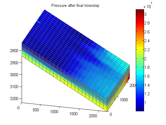
Plot pressure before and after schedule

We plot the pressure after the very first timestep alongside the pressure after the final timestep. By scaling the color axis by the minimum of the final state and the maximum of the first state, we can clearly see how the pressure has dropped due to fluid extraction.

h1 = figure;
H₂ = figure;

p_start = states{1}.pressure;
p_end = states{end}.pressure;
cscale = convertTo([min(p_end), max(p_start)],barsa);

figure(h1); clf;
plotCellData(G, convertTo(p_start,barsa))
axis tight; colorbar, view(v), caxis(cscale);
title('Pressure after first timestep')

figure(H₂); clf;
plotCellData(G, convertTo(p_end,barsa))
axis tight; colorbar, view(v), caxis(cscale);
title('Pressure after final timestep')

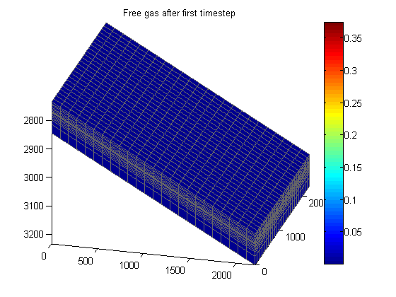
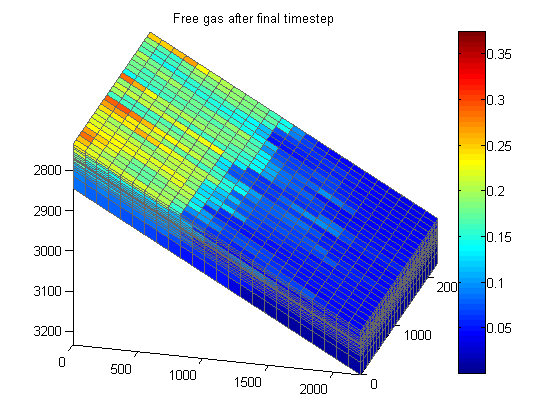
Plot free gas

Since the pressure has dropped significantly and we know that gas is being produced from the initially nearly saturated reservoir, we will look at the free gas. Again we consider both the first and the last state and use the same coloring.

sg0 = states{1}.s(:, 3);
sg = states{end}.s(:, 3);
cscale = [0, max(sg)];

figure(h1); clf;
plotCellData(G, sg0)
axis tight; colorbar; view(v); caxis(cscale);
title('Free gas after first timestep')

figure(H₂); clf;
plotCellData(G, sg)
axis tight; colorbar, view(v), caxis(cscale);
title('Free gas after final timestep')

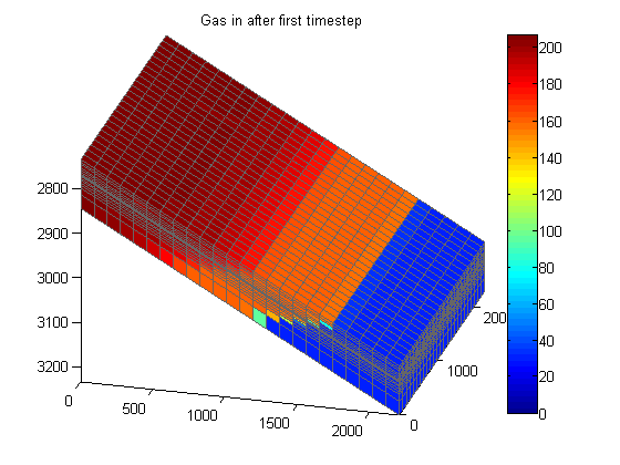
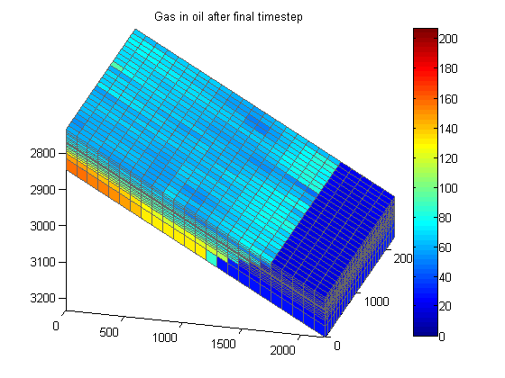
Plot dissolved gas

Since we did not inject any gas, the produced and free gas must come from the initially dissolved gas in oil (). We plot the values before and after the simulation, scaling the color by the initial values. Note that the values are interpreted as the fraction of gas present in the oil phase. As the fraction is calculated at standard conditions, the value is typically much larger than 1. We weight by oil saturations to obtain a reasonable picture of how the gas in oil has evolved. Plotting just the value is not meaningful if is small.

gasinoil_0 = states{1}.rs.*states{1}.s(:, 2);
gasinoil = states{end}.rs.*states{end}.s(:, 2);
cscale = [0, max(gasinoil_0)];

figure(h1); clf;
plotCellData(G, gasinoil_0)
axis tight; colorbar; view(v); caxis(cscale);
title('Gas in after first timestep')

figure(H₂); clf;
plotCellData(G, gasinoil)
axis tight; colorbar; view(v); caxis(cscale);
title('Gas in oil after final timestep')

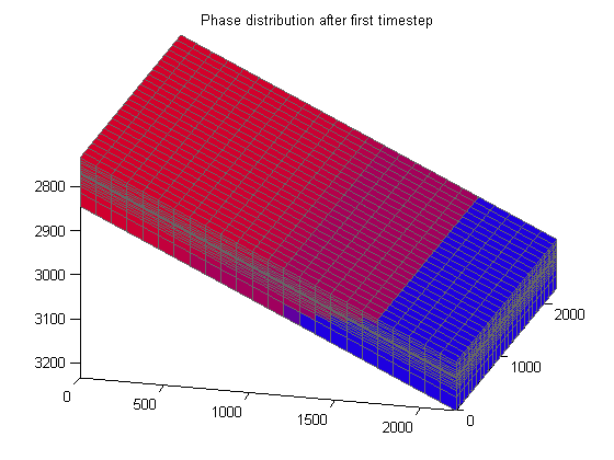
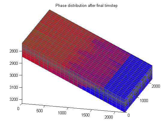
Plot phase distribution

s0 = states{1}.s(:, [2, 3, 1]);
s = states{end}.s(:, [2, 3, 1]);

figure(h1); clf;
plotCellData(G, s0)
axis tight; view(v)
title('Phase distribution after first timestep')

figure(H₂); clf;
plotCellData(G, s)
axis tight; view(v)
title('Phase distribution after final timstep')

Contents