Cross country skiing example with ActivityPresenter

Data from wearable microsensors such as inertial movement sensors (IMUs) are revolutionizing the analysis of movement. It allows researchers to bring the lab to the field, resulting in more relevant data for the analysis of movements in sports. However, there has been a lack of available tools to easily analyze the data. Especially, synchronizing the ground truth video of the movement of an athlete with the recorded data from microsensors has been challenging. SINTEF have developed an open source AutoActive Research Environment (ARE) [1] consisting of easy-to-use software with a graphical user interface, ActivityPresenter, to visualize, synchronize, and organize data from sensors and cameras as well as a supporting MATLAB and python toolbox. We demonstrate this software suite by sharing a dataset to analyze sub-techniques in classical cross country skiing as in [2]. 

We recorded data from IMU sensors mounted on the arm and chest and a video recording of a subject doing classical cross-country skiing. The raw accelerometer and gyroscope data was processed in MATLAB with cycles detected and labeled as described in [2]. The processed IMU data and cycle indications as well as sub-technique labels were synchronized with the video and written to an AutoActiveZip (aaz) file using the ARE MATLAB toolbox.

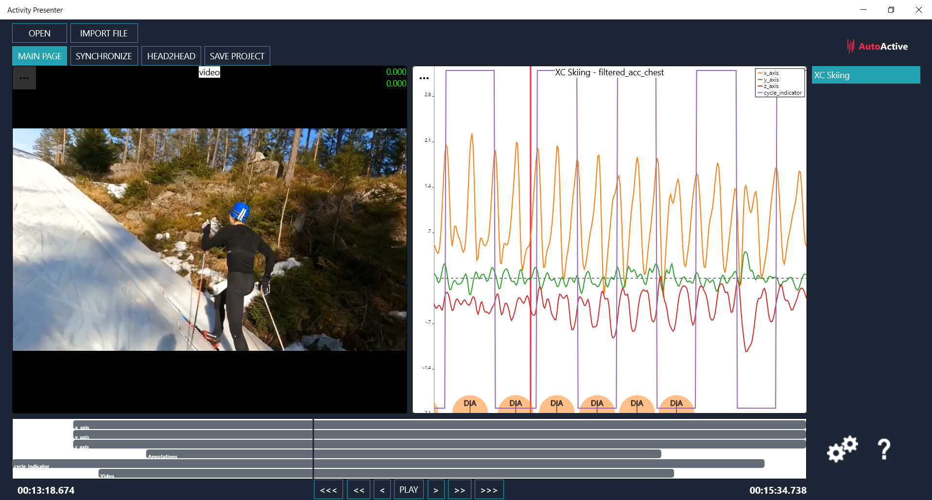
The processed data from the accelerometer on the chest is visualized in ActivityPresenter together with the cycle identification. Annotations are visible as DIA (diagonal) in the bottom of the plot. The data and video can be played as a movie or stepped through frame-by-frame. Additional annotations can be added by pre-selected keys per sub-techniques.

This example illustrates how to read and syncronize raw IMU data from Gaitup sensors, manipulate these data, and write the manipuated data syncronized with video and export this to a .aaz file to be visualized in ActivityPresenter. The example demonstrates first and foremost how to manipulate the data in MATLAB and how one can visualiz manipulated data in the ActivityPresenter.

Installation: To run this example, install the AutoActive ActivityPresenter and the AutoActive Matlab toolbox. Links and instructions for installation can be found here: https://www.sintef.no/projectweb/autoactive/software-platform/. The source code and data for this example is included in the Matlab toolbox installation.

Data: The data in this example is automatically downloaded, but can be manually downloaded from https://github.com/SINTEF/AutoActive-Matlab-toolbox/releases/download/v2.0.0_dataset/AutoActive_SampleData_xc_skiing.zip

Citationware: This code and data is citationware. If you use the data or code from this exampe you need to cite the following two papers:

Known issues when running this script:

Author: Ole Marius Hoel Rindal () Date: April 2022 Latest update: 23.01.2023.

Contents

Set up paths, download and unzip data

We will first set up the necessary paths for the toolbox and the physiolog MATLAB toolkit do be able to read the IMU data from the gait up sensors. The data and video used in this example is downloaded from the url below to the github repository.

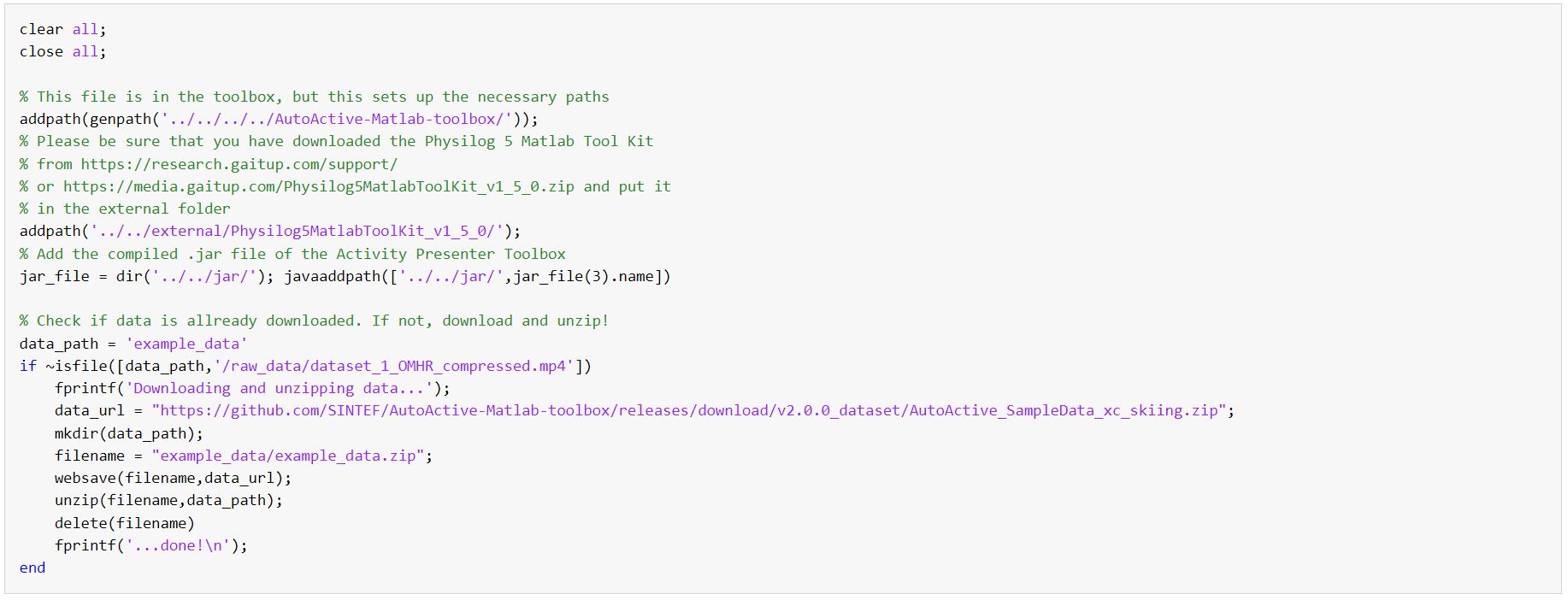
data_path =

    'example_data'

Read raw data from Gaitup Sensors

Read the raw IMU data from the .BIN files downloaded into MATLAB structs using the autoactive Gaitup plugin. NB! This is dependent on the Physilog5MatlabToolKit as specified in the paths above.

start reading gaitup data
%% Loading 2 Files %%
Reading : example_data/raw_data/0LA301.BIN
%%%% Reading Header %%%%
------- Physilog : ID = 1301 ---------
> Location : LA ---------
> Type : = 0 / Firmware = 1.2.6/ ---------
> Number of active sensors = 5 
>>> 1) accel / Fs = 256 Hz
>>> 2) gyro / Fs = 256 Hz
>>> 3) baro / Fs = 16 Hz
>>> 4) events / Fs = 256 Hz
>>> 5) radio / Fs = 256 Hz
%%%% Reading data %%%%
Reading part:1/1
Number of sectors: 1741 
>> 0 / 1741 sectors contain invalid data.
Missing sectors: 0 

Reading : example_data/raw_data/0ST283.BIN
%%%% Reading Header %%%%
------- Physilog : ID = 1283 ---------
> Location : ST ---------
> Type : = 0 / Firmware = 1.2.6/ ---------
> Number of active sensors = 5 
>>> 1) accel / Fs = 256 Hz
>>> 2) gyro / Fs = 256 Hz
>>> 3) baro / Fs = 16 Hz
>>> 4) events / Fs = 256 Hz
>>> 5) radio / Fs = 256 Hz
%%%% Reading data %%%%
Reading part:1/1
Number of sectors: 1696 
>> 0 / 1696 sectors contain invalid data.
Missing sectors: 0 

%% 2 Files sucessfully read %%
%%%% Synchronizing files %%%%
done reading gaitup data
start organizing gaitup data
done organizing gaitup data

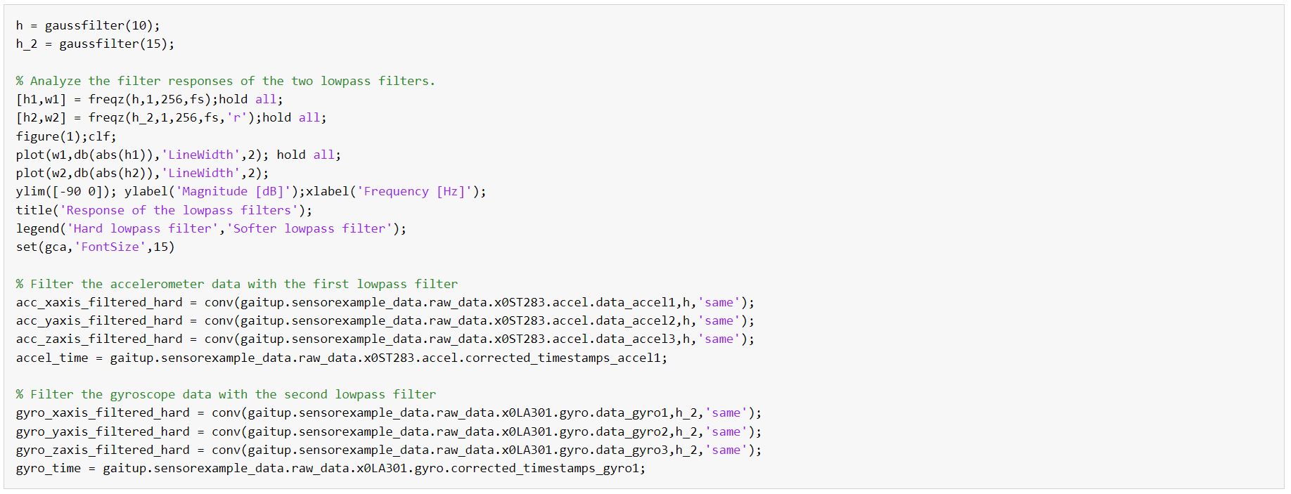
Filter data

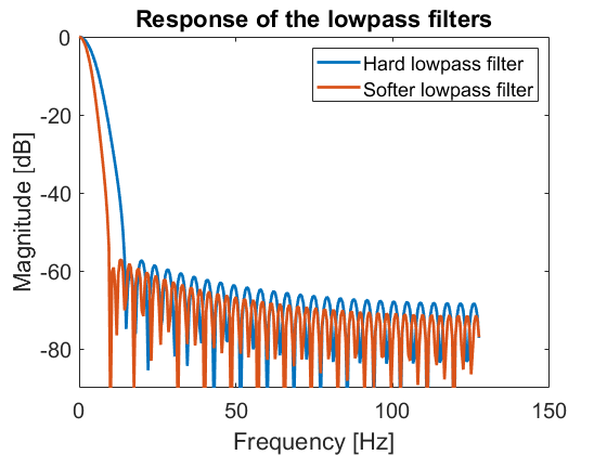
Create two Guasian filters with two different cutoff frequencies.

Detect cycles using gyro on arm

The cycles are detected by finding the peaks of the hard filtered gyroscope data from the arm. The peaks corresponds to the arm beeing exteded all the way behind the athlete.

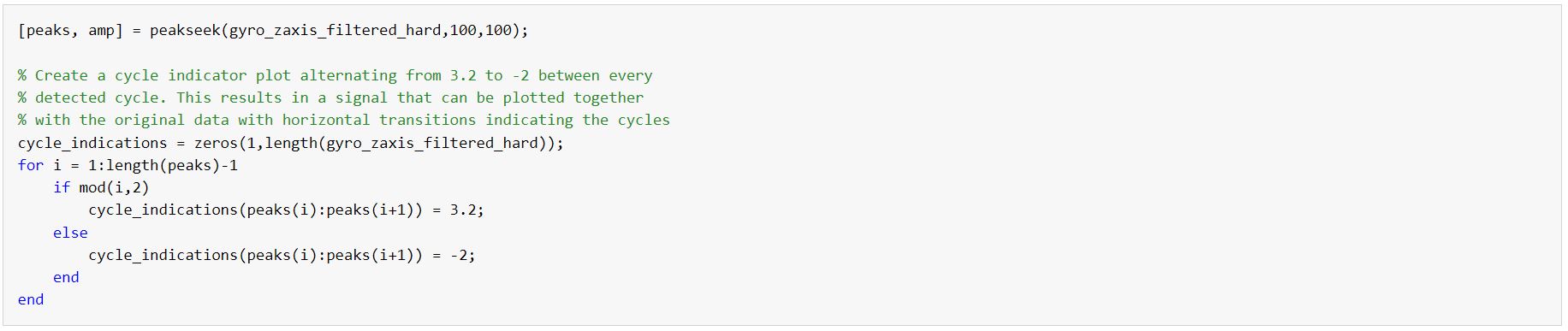
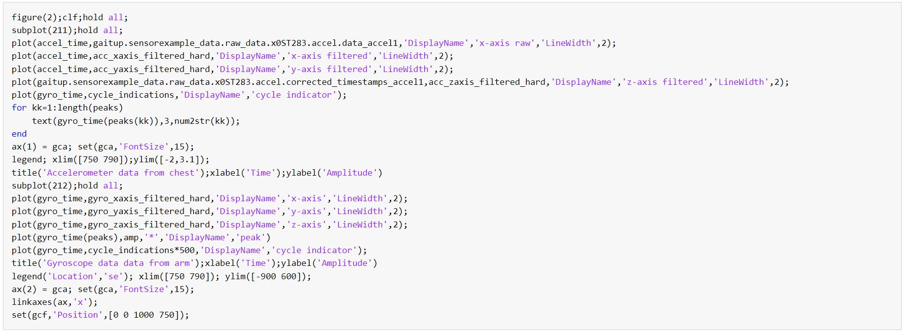
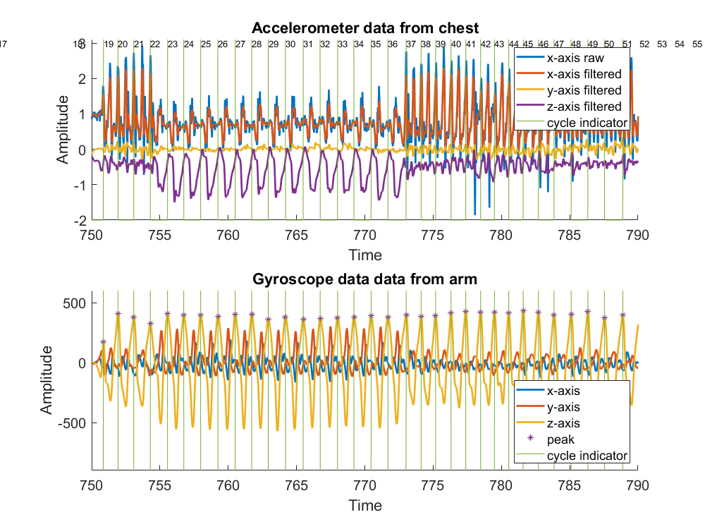
Plot result to investigate

Plot the accelerometer from the chest, both a trace of the unfiltered data as well as the filtered data from all axes. The cycles are indicated with horizontal lines as well as numbers to indicate each individual cycle. The second subplot si the gyroscope data from the arm, indicating the z-axis used to detect the cycles.

Create struct to be written to AutoActive Session

Create two structs to be written to the Auto Active Zip (aaz) file. The first struct is the cycle indication the second struct is the filtered accelerated data. The time in the structs are the syncronization between the signals.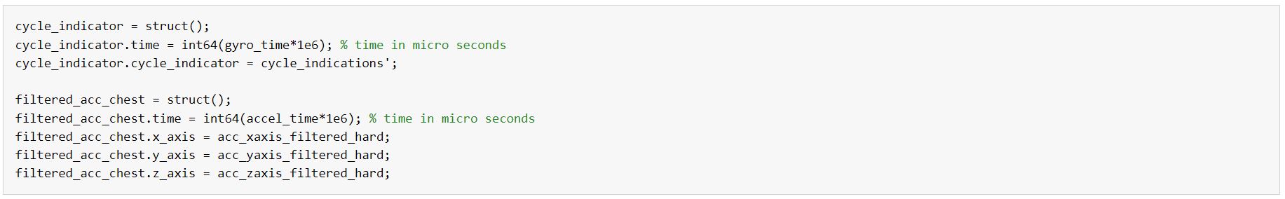

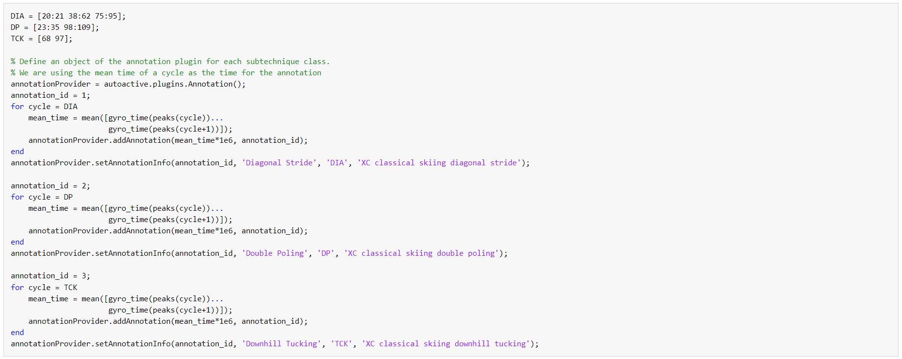
Add annotation

Based on the plot in Figure 2 we manually annotate the classical cross country skiing subtechniques. We will only annotate the cycles that are: * DIA = Diagonal Stride, annotation ID = 1 * DP = Dobbel Poling, annotation ID = 2 * TCK = Tucking (Downhill), annotation ID = 3

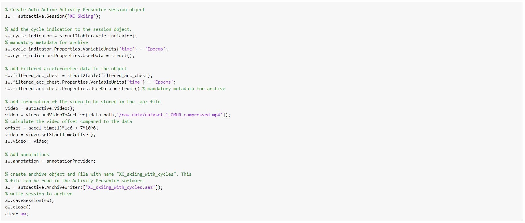
Write to Auto Active .aaz file

Finally, we are going to write the data we want to display in the Activity Presenter program in a Auto Active Zip .aaz file. We want to display the following data: + cycle indication + filtered accelerometer data from the chest sensor + synchronized video + annotations of type of sub technique for each cycle

ArchiveWriter <XC_skiing_with_cycles.aaz> - Open

Session <XC Skiing> - Writing data
autoactive.ArchiveWriter: Saving table <f2fb34ea-6abe-4720-a821-0bf5636cc99c/cycle_indicator.parquet>
autoactive.ArchiveWriter: Saving table <f2fb34ea-6abe-4720-a821-0bf5636cc99c/filtered_acc_chest.parquet>
Saving file to <f2fb34ea-6abe-4720-a821-0bf5636cc99c/video/dataset_1_OMHR_compressed.mp4>
autoactive.ArchiveWriter: Saving data <f2fb34ea-6abe-4720-a821-0bf5636cc99c/video/dataset_1_OMHR_compressed.mp4> from <example_data/raw_data/dataset_1_OMHR_compressed.mp4>
autoactive.ArchiveWriter: Saving textdata <f2fb34ea-6abe-4720-a821-0bf5636cc99c/Annotations/Annotations.json>
autoactive.ArchiveWriter: Saving metadata <f2fb34ea-6abe-4720-a821-0bf5636cc99c/AUTOACTIVE_SESSION.json>
Session <XC Skiing> - End
autoactive.ArchiveWriter: ArchiveWriter <XC_skiing_with_cycles.aaz> - Closing

Implementation of the Gaussian lowpass filter used

The lowpass filter used in this is example is included for simplicity. It is a simple Gaussian lowpass filter used at two different cutoff frequencies.

Published with MATLAB® R2020a