Hjem til forsiden

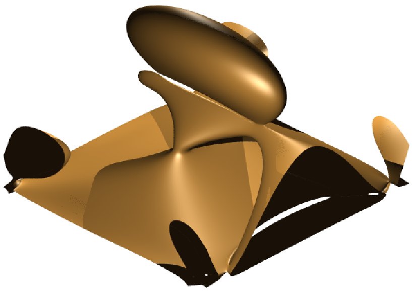
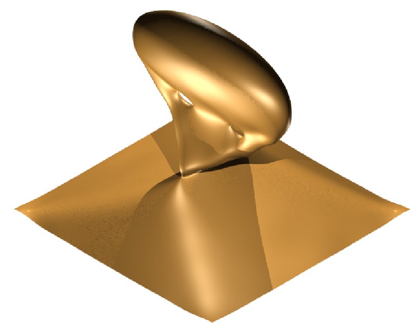
Approximate implicitization by point sampling & normal estimates

This method for approximate implicitization has been developed at Linz. It is characterized by the simultaneous approximation of sampled point data Pi (xi, yi, zi) and estimated normals  ni  at these points. The method produces an approximate implicit representation of the form f(x, y,z) = sum (Ci  Bi(x, y, z)) with basis Bi(x, y, z) and a certain coefficients Ci

The points Pi (xi, yi, zi)   are organized into segments. The segmentation is realized by a simple region growing process. Simultaneously while building the segments we propagate the orientation of the estimated normals. This is simply done by checking the scalar product of the normal of the point which is to be added and the normal of the closest point that already belongs to the segment. If this product is negative, then the orientation of the normal is needs to be swapped. In order to control the shape of the resulting surface, an additional tension term is optimized. It pulls the approximating surface towards a simpler shape. The implicit function is obtained as the minimum of a convex quadratic objective function


sum  f(xi, yi,zi)2  +  w || grad(f(xi, yi,zi)) - ni ||2  + ``tension''


where w is a positive weight controls the influence of the estimated normal vector ni  to the resulting surface. This method is fully general, i.e., it can be applied to any space of functions, not only to piecewise polynomials. For practical applications, however, fast evaluation of basis functions is important. For this reason we implemented the algorithm for trivariate tensor-product B-splines. In this case, the basis functions ensure global smoothness, and the resulting system of linear equations is sparse.

Choice of the spline space

The domain of interest is divided into cubes of the same size. This is done by specifying a cell-size. In order to guarantee an integer number of cells, the bounding box of the input surface is enlarged a bit. The domain of the spline functions consists only of the ``active cells'', i.e cubes that containing data, and its neighbors. Another input parameter is the degree d of the spline function. We choose the knot vector with simple knots in the interior, so the continuity is Cd-1.

Due to the compact support of the B-splines, the implementation is relatively fast because of the sparsity of the resulting linear system of equations. Consequently, even complicated singular surfaces can be implicitized. The figure below shows a surface with two self-intersecting curve. It has been approximately implicitized by tetrahedral polynomial (left), tensor product polynomials (middle) and tensor product spline (right). By using spline functions, one may avoid unwanted branches completely.


Published June 23, 2005

Examples of approximation

Nested nodal tetrahedral

Approximated by tetrahedral polynomial missing parts and giving extra branches.

nested nodal tensor

Approximated by tensor product polynomial giving extra branches.

Nested nodal spline

Appoximated by tensor product spline giving no extra branches.