![\[\frac{\partial I}{\partial t} = R\]](form_113.png)
Here,  represents the image, while
  represents an (image-dependent) smoothing term to be further specified.
 :
:
![\[E(I) = \int_\Omega ||\nabla I||^2 d\Omega\]](form_115.png)
Which, through the use of the Euler-Lagrange equation gives us the following PDE (the heat equation):

This smoothing process is isotropic; it smooths with equal strength in all spatial directions. This means that edges in the image will soon become blurred. In LSSEG, we can apply this smoothing scheme by calling the nonlinear_gauss_filter_XD() function and setting the parameter p equal to zero.
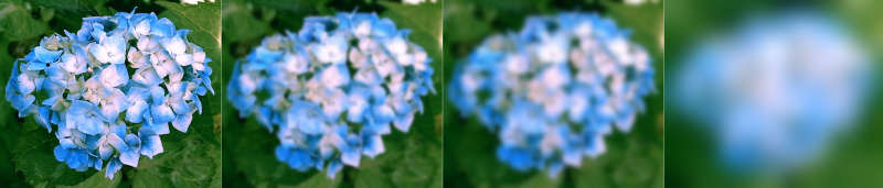
Example of progressive smoothing of an image using the heat equation
![\[E(I) = \int_\Omega ||\nabla I|| d\Omega\]](form_116.png)
We see that it is somewhat similar to the integral in our last example, except that we have not squared the norm. This functional measures the total variation of the image, and the PDE we obtain from the Euler-Lagrange equation describes a process we call total variation flow. This process has several interesting theoretical properties; readers are refered to section 2.1.1 of Brox' thesis for an overview of these, and to section 2.3.2 to 2.3.4 of the same thesis for an examination of the resulting PDE. As for the previous example, the limit of the smoothing process is a constant image (and we will arrive there in finite time). However, the intermediate images are quite different. The edges in the image are well preserved for a long time, regions gradually merge with each other, and the intermediate images take on a segmentation-like appearance. The PDE system is:
In LSSEG, we can apply total variation flow on an image using the function nonlinear_gauss_filter_XD() with the parameter p equal to 1.
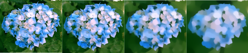
Example of progressive smoothing of an image using total variation flow
![\[\frac{\partial I}{\partial t} = div\left(g(||\nabla I||) \nabla I\right) \]](form_118.png)
with  a scalar function that is 1 in the first example and
  in the second. Without departing from a functional, we can create customized schemes by specifying this function
  directly. What we want is to slow down diffusion in regions with high gradients (i.e., edges) while still allowing diffusion to take place at normal speed in "flat" regions. This idea was put forward by Perona and Malik in 1990, where they proposed the following choice of :
![\[g(||\nabla I||) = \exp\left(-\frac{||\nabla I||^2}{K^2}\right)\]](form_122.png)
 is here a fixed threshold that differentiates homogeneous regions from regions of contours. Tschumperle gives a good theoretical explanation of this in section 2.1.2 of his thesis, where he also shows that not only does this process lead to smoothing whose strength depend on the local gradient; it also smoothes with different strength (which can be explicitely determined) along the local image gradient and isophote.
is a scalar function that only depends on the image gradient norm. A more general formulation would be:
![\[\frac{\partial I}{\partial t} = div\left(D \nabla I\right)\]](form_124.png)
where  is a tensor field defined on the domain and with values in the space
  of tensors described by positive-definite 2x2-matrices. (In case of three-dimensional images, i.e., volumes, we use
  instead of ). We call
  a field of diffusion tensors. Contrary to described above, depends not on the image gradient itself, but rather on the position in the image . Moreover, as
  is a tensor rather than a scalar, its effect on the smoothing term also varies with the local direction of
  (matrix-vector multiplication
  ). The smoothing at position
  will in general be strongest along the direction specified by the eigenvector with largest eigenvalue of , and weakest in the direction specified by the other eigenvector (which, due to the symmetry of the matrix, is perpendicular on the first). See the section on definition of a smoothing geometry for more on how the tensor field can be specified. For more on divergence-based PDEs, refer to section 2.1.4 of Tschumperle's thesis.
inside the  term leads to a term which depend on the derivative of . For this reason, we cannot in general say that the smoothing process locally follows the directions specified by the tensor field . D. Tschumperle shows that a more "predictable" process can be obtained by using the smoothing geometry in a trace-based formulation:
![\[\frac{\partial I}{\partial t} = trace(TH) \]](form_134.png)
Here,  is the smoothing geometry and
  is the local Hessian matrix of the image. For more details on this equation, and a discussion about how it differs from the divergence- based formulation, please refer to 2.1.5 and section 2.4.1 respectively of Tschumperle's PhD-thesis. In section 3.2.1 of the same thesis, Tschumperle shows that this equation has an analytical solution which is:
![\[I(t) = I_0 * G^{(T, t)}\]](form_136.png)
Where  is the original image,
  is the image at time
  of the evolution process, and
  is a bivariate oriented Gaussian kernel:
![\[ G^{(T, t)}(x) = \frac{1}{4\pi t}\exp\left(-\frac{[x,y]T^{-1}[x,y]^T}{4t}\right)\]](form_141.png)
in the image. Typically, in regular areas of the image, we want to smooth equally in all directions, whereas in regions with important gradients, it is important to smooth the image in a way that does not destroy the gradient, i.e., smooth much less along the gradient than in the direction perpendicular to it (the isophote direction). Thus, in order to define the smoothing geometry tensor field, we should, for each point in the image, define two directions (2D-vectors) and the smoothing strength along these who directions (scalars). In order to define these, we base ourselves on a smoothed version of the image's structure tensor. (The reason we smooth the structure tensor is to determine a gradient for each pixel that is somewhat less "local", thus representing structures in the image that go beyond the size of one pixel and also obtaining gradient estimates that are more robust against image noise).
For a given image point , the eigenvectors of the structure tensor represent the two privileged smoothing directions. Due to the smoothing of the structure tensor, we cannot directly refer to these eigenvectors as the gradient and isophote of the image at , but they are perpendicular and represent the direction along which the image varies the most (and thus were we should smooth little) and the direction along which the image varies the least (and thus where we should smooth more). The corresponding eigenvalues give information about strong the variation is. If the two eigenvalues are identical, then the image variation around this point is more or less the same in all directions, and the smoothing geometry should be isotropic here. If the two eigenvalues are different, we should smooth more along the direction with the smaller eigenvalue than along the direction with the bigger one, and the difference in smoothing strength (the anisotropy) should be reflected by the difference between these two values. If we name the two directions  and
and  , and choose two corresponding smoothing strenths
  and
and  , the smoothing geometry matrix representation for a given image point becomes:
![\[T = c_1 u u^T + c_2 v v^T\]](form_142.png)
In LSSEG, we have a function called compute_smoothing_geometry_XD() that computes a smoothing geometry based on an image's structure tensor. Here, the two smoothing directions and are the eigenvectors of the structure tensor, and the corresponding smoothing strengths are taken to be:
![\[c_1 = \frac{1}{(1 + \lambda_u + \lambda_v)^{p_1}}\;,\;\;\;\;c_2 = \frac{1}{(1 + \lambda_u + \lambda_v)^{p_2}} \]](form_15.png)
where  and
and  are the two eigenvalues of the structure tensor corresponding to and respectively. This choice is discussed briefly in section 2.1 of [Tschumperle06]. Note that as long as
  , then the smoothing will be stronger along direction than along direction , and this difference will be more pronounced as the biggest eigenvalue (an thus the denominator of the fractions above) grows.
. This does a good job in preserving edges, but on curved structures, especially sharp corners, this leads to an undesirable rounding effect. The problem is that the gaussian kernel does not take curvatures into account. As a remedy, Tschumperle proposes an approach which can be seen as local filtering of the image with curved gaussian kernels . He develops the theory and algorithm in section 3 and 4 of his paper Fast Anisotropic Smoothing of Multi-Valued Images using Curvature-Preserving PDE's. In short, he splits the smoothing geometry tensor field into a sum of vector fields, and then performs line integral convolutions of the image with each of these vector fields and a univariate gaussian kernel function:
![\[G_t(s) = \frac{1}{4t}\exp\left(-\frac{s^2}{4t}\right)\]](form_144.png)
is here the timestep used. In other words he carries out 1-dimensional convolutions of the image with  along the streamlines defined by the vector fields obtained from .
in the following way:
![\[T = \frac{2}{\pi} \int_{\alpha = 0}^\pi (\sqrt{T}a_\alpha)(\sqrt{T}a_\alpha)^T\]](form_146.png)
where ![$a_\alpha = [\cos \alpha, \sin \alpha]^T$](form_147.png) and
and  is a tensor field that is the "square root" of , in the sense that
  . If
. If  , then
 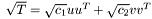 .
.
![\[\frac{\partial I}{\partial t} = trace(TH) + \frac{2}{\pi}\nabla I^T \int_{\alpha=0}^\pi J_{\sqrt{T}a_\alpha}\sqrt{T}a_\alpha d\alpha\]](form_152.png)
where  stands for the Jacobian of the vector field
  . However, the system is not solved using the "standard" method of discrete differencing on a regular grid. Instead, he demonstrates how this can be interpreted as a combination of 1D heat flows along the streamlines of the various vector fields
  .
.
image smoothed using our implementation of Tschumperle's algorithm. The parameters are the default ones, and the number of timesteps are 1, 4 and 8 (original image to the left)
 1.4.7
1.4.7