A glossary of a few selected terms as used in this documentation

Anisotropic smoothing
In short, anisotropic smoothing of an image, as opposed to isotropic smoothing, is some kind of regularization process that does not smooth the image equally in all directions. One of the earliest schemes for anisotropic image smoothing was Perona and Malik's regularization, which you can read a short presentation about in section 2.1.2 of D. Tschumperle's PhD thesis.

By an image channel
we mean one of the image components. Each pixel in the image contains one separate value for each image channel. For instance, a color image usually has at least three separate channels, one for its red component, another for its green and a third for its blue. Channels do not conceptually need to represent colors though. the LevelSetFunction class, which inherits from the Image class, always contains exactly one channel, which represents the value of the level-set function for each pixel position. A Mask is another kind of single-channeled image, where the channel value per-pixel is boolean and represents whether or not that pixel is active or masked out .

A diffusion tensor
in 2D is a tensor described by a symmetric, semi-definite, positive 2x2 matrix (3x3 in 3D). It is used in smoothing partial differential equations, and describes the amount of diffusion along privileged spatial directions. The matrix has two real eigenvalue/eigenvector pairs, its eigenvectors are perpendicular. The eigenvectors describe two spatial directions, and their respective eigenvalues represent the amount of diffusion along these directions. If we denote its eigenvalues $\lambda_1, \lambda_2$ and the corresponding eigenvectors , the diffusion tensor can be decomposed into:
$T = \sum_{i=1}^2 \lambda_i u_i u_i^T$

The Euler-Lagrange equation
The Euler-Lagrange equation is the major formula of the calculus of variations. It can be considered the gradient of a functional, and gives a necessary condition that must be verified for a function that minimizes the functional. For functions over an -dimensional domain $\Omega$ , and for a functional
$J(f)=\int_\Omega F(f, x_1, ..., x_n, f_{x_1}, ..., f_{x_n}) d\Omega$
the corresponding Euler-Lagrange equation is given by:
$\frac{\partial F}{\partial f} - \sum_{i=1}^n \frac{\partial}{\partial x_i}\frac{\partial F}{\partial f_{x_i}} = 0$
As the right-hand side of the equation above can be considered the gradient of , we can use it in a way analog to function minimization by gradient descent. In this way, we look for a minimum of by iteratively taking steps going "downhill" until the gradient vanishes. We introduce an "artificial" time parameter, then start from an initial function and following the opposite direction of the gradient until we arrive at a local minimum of . This leads to the following partial differential equation evolution process:
$\begin{eqnarray*} f_{t=0} &=& f_0 \\ \frac{\partial f}{\partial t} &=& - \left(\frac{\partial F}{\partial f} - \sum_{i=1}^n\frac{d}{d x_i}\frac{\partial F}{\partial f_{x_i}}\right) \ \end{eqnarray*}$

A functional
is, for our purposes, a function that takes functions (from some specified class) as its argument, and return a scalar value. We are often interested in the functions for which a given functional reaches a minimum. It is typically defined by an integral. For functions over a domain $\Omega$ , this can be written
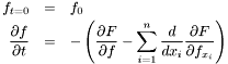
$J(f) = \int_\Omega F(x, f(x), \nabla f(x), ...)d\Omega$
where is a function of the position in $\Omega$ , the value of and its derivatives (possibly also higher-order) at this position. In the process of searching for a minimum of a given functional, we often make use of the Euler-Lagrange equation.

The heat-equation
is a partial differential equation that is the simplest form of the diffusion equation. It is much used in physics to describe diffusion of a quantity through an isotropic medium, like heat through a solid. If is the function describing the quantity, the equation can be written:
$\begin{eqnarray*} I_{(t=0)} & = & I_0 \\ \frac{\partial I}{\partial t} & = & \Delta I \end{eqnarray*}$

the Hessian matrix
of a function $f : R^2 \rightarrow R$ is defined by the second derivatives and cross derivatives of :
$H(x,y) := \left[ \begin{array}{cc} \frac{\partial^2 f}{\partial x^2} & \frac{\partial^2 f}{\partial x \partial y} \\ \frac{\partial^2 f}{\partial x \partial y} & \frac{\partial^2 f}{\partial y^2} \end{array} \right]$

A level-set function
is, in our terminology, a scalar function $\phi$ defined on some domain $\Omega$ and which is used to define a partitioning of the domain into two regions separated by a boundary defined by its zero set. Hence, $\phi$ takes on positive value for one region, and negative for the other. The boundary curve is implicitly defined by the level-set curve. On the other hand, for any given closed curve in $\Omega$ , we can define a level-set function that represents it. A common way of doing that is by letting the level-set function be the signed distance function of the curve. Level-set functions is defined in LSSEG by the class LevelSetFunction, which is a very central data structure.

Line-Integral-Convolution (LIC)
Given an image, a vector field defined on the same domain $\Omega$ as the image, and a kernel function $k : \mathbf{R} \rightarrow \mathbf{R}$ , we define the line-integral-convolution as the one-dimensional convolution of the image with the kernel function along all streamlines defined by the vector field. This results in an image that is smoothed along those streamlines. This technique is useful for visualizing a vector field (by convoluting an image consisting only of noise with a gaussian kernel along the streamlines of the field), but also for curve-preserving smoothing schemes of images (in which case the vector field has been determined based on structures present in the original image). Refer to [Cabral93] for details on the process, and to [Tschumperle06] for this technique used for curve-preserving smoothing.

Mean curvature motion
is a motion of an interface (boundary curve, surface) along its normal direction, with a velocity proportional to its curvature. It can generally be described by the equation:
$\overrightarrow{V} = -b\kappa \overrightarrow{N}$
where $\overrightarrow{V}$ is the velocity vector, , $\overrightarrow{N}$ is the normal vector and $\kappa$ is the curvature. In a level-set formulation, where the interface is described by a level-set function, this equation can be written:
$\frac{\partial\phi}{\partial t} = b\kappa |\nabla\phi|$
where $\phi$ is the level-set function and $\kappa = \nabla . \left(\frac{\nabla\phi}{|\nabla\phi|}\right)$ is the curvature of the isocurves of $\phi$ . The full formulation is therefore:
$\frac{\partial\phi}{\partial t} = b \nabla . \left(\frac{\nabla\phi}{|\nabla\phi|}\right) |\nabla\phi|$
Numerically, this can be discretized using central differencing (as decribed by [Osher03]. In order for the integration to be stable, the timestep $\Delta t$ must respect the following CFL-condition (on a 2D domain):
$\Delta t\left(\frac{2b}{(\Delta x)^2} + \frac{2b}{(\Delta y)^2}\right) < 1$
Motion by mean curvature is described in chapter 4 of [Osher03].

The Mumford-Shah functional
is an energy functional used in the context of image segmentation. For a given partitioning of an image into region, and a given approximation of the original image in those regions, it gives a numerical value that measures the "goodness" of that particular partitioning. This value takes into account the difference between the approximated image and the original one, as well as how regular the proposed approximation is and how long the combined length of boundaries. Lower values of this functional means a better segmentation, and for that reason, image segmentation often becomes the matter of searching for minima of this functional. In its full form, it can be written:
$E(u, \Gamma) = \int_\Omega (u-I)^2 dx + \lambda \int_{\Omega - \Gamma} |\nabla u|^2 dx + \nu\int_\Gamma ds$
Here, $\Gamma$ represent the partitioning of the image domain $\Omega$ into distinct regions, whereas is a smooth approximation of the image within each region (it is allowed to be discontinuous across region boundaries, though). The first term on the right side measures the distance between the approximated image and the origional image . The second term on the right side measures the regularity of within each region. The last term on the right side measures the total length of the boundaries separating the regions. $\lambda$ and $\nu$ are tuneable weighing terms describing how much importance to give to the second and third right-hand-side term compared to the first.

The normal direction flow
is referred to here as a motion of an interface (boundary curve, surface) along its normal direction, vith a velocity imposed from outside. We suppose that this motion does not depend on the interface, but it can depend on the spatial coordinate. In the level-set formulation, where the interface is described by the zero-set of a level-set function $\phi$ , the formula is:
$\frac{\partial\phi}{\partial t} + a|\nabla\phi| = 0$
(Here, might vary over the domain, although it is not dependent on $\phi$ ). This is an example of a Hamilton-Jacobi equation, and must be discretized accordingly. In order to assure stability, the timestep used must then fulfill the following CFL condition (on a 2D domain):
$\Delta t \max\left\{\frac{|H_1|}{\Delta x} + \frac{|H_2|}{\Delta y}\right\} < 1$
where and are the partial derivatives of the systems Hamiltonian with respect to $\phi_x$ and $\phi_y$ . (The Hamiltonian of this equation is $H(\nabla\phi) = a|\nabla\phi|$ ). Motion in the normal direction is described in chapter 6 of [Osher03], although there, does not vary over the domain. The theory of Hamilton-Jacobi equations and their numerical discretization is introduced in chapter 5 of the same book.

A normal force field is a field of scalars defined over the domain of a level-set function $\phi$ , representing a force acting normally on the level-set curve (surface in 3D) of $\phi$ at that particular point. Normal force fields are used to evolve level-set curves (surfaces) over time, and are determined using ForceGenerators.
Note:
Since a normal force field can be seen as a single-valued image over the domain, in the LSSEG library we represent it using another LevelSetFunction (not to be confused with the LevelSetFunction used to represent the actual segmentation).

Reinitialization of a level-set function
During the segmentation process, the level-set function undergoes an evolution based on a partial-differential equation. What interests us is where the level-set function is negative, where it is positive and where it is zero (i.e. its zero set). Beyond that, its exact numerical values are generally not of interest for us. However, during the evolution, the level-set function can develop regions that are very flat or very steep, which might stall the process due to increasingly shorter stable timesteps, or other numerical problems. For that reason it is desireable to reset the level-set function to a signed distance function once in a while. The signed distance function in question should have same zero-set and sign as the original level-set function, but having a gradient of 1 almost everywhere, it leads to a much more stable evolution process afterwards.

The scale measure
as defined by Thomas Brox in section 4.1.2 of his thesis, is used in the context of texture discrimination for image segmenting purposes. It is a single-channeled image derived from the image to be segmented, and whose pixel values give an estimate of the scale of the structure that the corresponding pixels in the original image are part of. The computation of this measure is based on a total-variation-diminishing flow, and is somewhat technical. The reader is referred to the relevant section of Brox' thesis for all the details.

The signed distance function of a closed contour in a 2D domain or a closed surface in a 3D domain, is the function that assigns to each point in the domain its shortest distance to the contour/surface, with a sign that indicates whether the point is situated inside or outside the enclosed domain. In our implementation, we have chosen the convention that negative values signifies the inside. The zero-set of a signed distance function is exactly the closed contour/surface we started out with.

The structure tensor
of an image is a tensor field over the image domain $\Omega$ . In each point of $\Omega$ , the tensor describes the orientation of local structures in the image around this point. It is represented by a symmetric, positive, semi-definite 2x2 matrix. For greyscale images, this matrix, , is defined by (subscripts of denote partial derivatives):
$G_0(x,y) := \nabla I\nabla I^T = \left[ \begin{array}{cc} I_x^2 & I_xI_y \\ I_xI_y & I_y^2 \end{array} \right]$
For multi-channel images (e.g., color images) with N channels, the definition is:
$G_0(x, y) := \sum_{i=1}^N \nabla I_i \nabla I_i^T$
For various reasons, we often prefer to work with the smoothed structure tensor $G_\rho$ instead. This is obtained through convolution with a Gaussian kernel:
$G_\rho : = G_0 * K_\rho$
Much useful information about the structure tensor can be found in section 2.2 of Brox's PhD thesis.

The zero-set of a level-set function is the ensemble of points in its domain for which the function evaluates to zero.

Generated on Tue Nov 28 18:35:47 2006 for lsseg by

1.4.7