GeoScale - Direct Reservoir Simulation on Geocellular Models

Corner-point grids
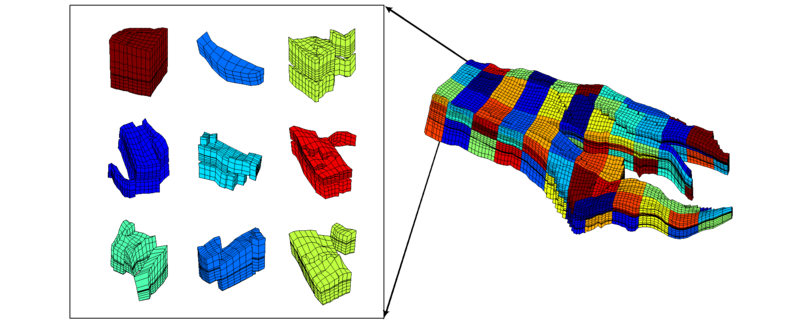
The multiscale method is very robust with respect to the coarse grid. For corner-point grids, the simplest, and most accurate, method to generate a coarse simulation grid is by a regular partitioning in index space (i.e., using the logical ijk numbering of the grid cells). This way, one can make sure that the coarse blocks follow the geological structures in the grid and obeys the modelling assumptions used to build the model. Equally important, using a partitioning in logical space enables the coarsening to be automated in a straightforward manner.

Key steps in the multiscale method

  1. First we introduce a coarse grid for which each block consists of a connected collection of cells from the underlying fine grid, as seen in Figs 1 and 2a. For corner-point grids the simplest and yet most effective approach is to partition the input grid in index-space, using e.g., a uniform partitioning in which each coarse block is assigned an equal number of cells in index space. This may give highly irregular block geometries, as seen in Fig. 2a, but preserves geological structures, simplifies the coupling in the resulting linear system, and most importantly, enables automatic coarsening of grids. We refer the reader to Aarnes et al. (2008) for a more thorough discussion and some simple guidelines on how to generate good coarse grids.
  2. Next, we detect all pairs of adjacent gridblocks, as illustrated in the third subfigure of Fig 1.
  3. For each pair of adjacent gridblocks, we solve a local flow problem numerically to determine basis functions, as shown in Figs 1 and 2b, that will later be used as building blocks for constructing the global solution; see Figs 1 and 2c. The exact formulation and discretization of the local flow problems is discussed in full detail in the next section.
  4. For each time-step in the simulation we:
    • Check if any basis functions require recomputing; more details about this later.
    • Assemble the coarse-grid system using the variational form from the corresponding mixed finite-element formulation, which amounts to integrating multiscale basis functions and computing their interaction. In a practical implementation, this is done by matrix vector multiplication, as will be explained in more detail in the next section.
    • Recover pressures and velocities/fluxes on the underlying fine grid. This is achieved directly using the subgrid resolution in the multiscale basis function.
    • Solve the fluid-transport equations using the fine-scale pressures and fluxes, which are assumed to be constant in time.

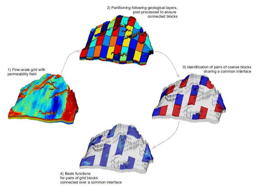
Fig 1: Key steps in the multiscale method illustrated for a model from the SAIGUP study.

Fig 1a: Introduce a coarse grid by partitioning the input grid in index space, as seen in the right plot. The left plot shows a selection of nine coarse gridblocks.

Fig 1b:The left plot shows the velocity magnitude for a basis function modeling flow between the two adjacent gridblocks depicted in the bottom right plot. In the top right plot we show the logarithm of the corresponding permeability field.

Fig 1c: A selection of velocity basis functions shown in the global reservoir model. All basis functions model fine-grid flow patterns between two adjacent gridblocks. The MsMFE velocity solution is expressed as a linear superposition of all velocity basis functions.

Published September 17, 2009

A portfolio of strategic research projects funded by the Research Council of Norway