How Segmentation in LSSEG Works

The theory behind the level-set based segmentation approach used by LSSEG is thoroughly explained in chapter 4 and 5 of Thomas Brox' PhD thesis. The reader is strongly recommended to read at least these two chapters, as the passages below only are intended to give some general idea about what is going on.

Overall explanation of problem

When we talk about segmentation of an image, we mean a way to partition the image into different regions in some meaningful way. Generally, we want to separate parts of the image that belong to different objects. When attempting to do this in an automatical fashion, we run into the problem that a computer does not have any direct way of recognizing physical objects. For that reason, we define segmentation algorithms that divide the image into regions which are similar in some specifiable way, and try to make this correspond as well as possible with the actual image semantics.

The way we work, we try to define regions whose boundaries are somewhat regular, and in a way such that the pixel distribution of each region has distinct statistical properties.

How regions are represented - level set functions

If we want to separate an image into regions, we need some way to represent a region, ie. a way to specify which of the image pixels that are contained within the region. A region does not necessarily need to be connex (it can consist of multiple disjoint parts) and its topology can include handles and holes.

In this library, we use level-set functions to represent regions. They are very flexible in that they allow for arbitrary topology of regions, are easy to modify and as (differentiable) functions they fit well into a PDE framework.

A level-set function is a scalar function defined over the whole image domain, and defines a separation of the image into two parts: those parts of the image where the level-set function takes on a negative value is defined as being a separate region from those parts where the level-set function takes on a positive value. In LSSEG, we choose the convention that all parts of the image domain where the level-set function is negative is called the interior of the region represented by the level-set function (all the rest thus constituting the exterior). Also, those parts of the image where the level-set function is zero is called the boundary of the domain.

in LSSEG, the level-set function is represented by the class LevelSetFunction. This class inherits from the Image class and can thus be regarded as a (greyscale) image itself; each of its pixels representing the value taken on by the level-set function at the position of that pixel. (NB: the LevelSetFunction has a restriction not present in its base class Image: it always has exactly one channel).

For a very good book on level-set functions and their use, refer to [Osher03].

changing the shape of a region described by a level-set function

In the segmentation process described here, we obtain our final partitioning of the image by starting from some initial partitioning, which we change in a continuous way in order to arrive at the region(s) (hopefully) sought. This is done by developing the level-set function describing a region, according to a time-dependent partial differential equation that incorporates information taken from the image. So how can we change a region using a time-dependent partial differential equation? We will here describe two basic equations we use, and the effect that they have on a region described by a level-set function $\Phi$ . Remember our convention that the interior of the region described by our level-set function is the domain on which the level-set function is negative, and that the boundary of this region is described by the domain on which the level-set function is exactly zero (a curve, except in degenerate cases). Again, refer to the book by Osher for formal explanations and additional detail.

mean curvature motion The main effect of mean curvature motion is to shrink the interior region and smoothen its boundary curve. If mean curvature alone is allowed to act on a (closed) region described by a level-set function, this region will eventually shrink until it disappears. The partial-differential equation is: $\partial_t \Phi = |\nabla\Phi|div(\frac{\nabla\Phi}{|\nabla\Phi|})$ . Discretized, this describes the change in $\Phi$ from one timestep to the next. In the LSSEG library, the quantity $|\nabla\Phi|div(\frac{\nabla\Phi}{|\nabla\Phi|})$ can be directly obtained from a LevelSetFunction through use of the member function LevelSetFunction::curvatureTimesGradXD(). Note that movement by mean curvature motion is completely determined by the shape of the level-set function itself, and is not influenced by any external factors.

normal direction flow The effect of normal direction flow is to push the boundary curve outwards / pull the boundary curve inwards along its normal in each point. The magnitude of this "push" can vary over the domain, and in our segmentation process, this magnitude is governed by information taken from the picture. The partial differential equation is: $\partial_t\Phi = \beta \dot |\nabla\Phi|$ Here, $\beta$ may vary over the domain, hence the effect on $\Phi$ is not the same everywhere, which allows for controlling its development according to external factors. The incremental change in the level-set function due to normal direction flow can be computed in the LSSEG library by using the functions normal_direction_flow_XD(). In order to define a $\beta(x,y)$ function to use in segmentation, we use ForceGenerators.

In the segmentation process of this library, these are the two only kinds of movement tools necessary.

Note:

It might be not be intuitive to associate the movement of a boundary curve with the development of a level-set function. In order to see this clearer, the reader should consult the book by Osher, or read section 5.1 of Brox' thesis.

Applying any of the above differential equations on $\Phi$ is quite computationally expensive. However, we are only interested in the development of $\Phi$ around its current zero-set, where the current region boundary is located. Therefore, we only apply the above equations to a small band along this boundary. Since this boundary will move over time, the band will move along with it. All parts of the level-set function away from this band will be left as it is (except that it may be occationally reinitialized to the signed distance function).

Specifying a segmentation criterion - the Mumford-Shah functional

In order to partition our image into regions, we need to specify what we are trying to obtain. As we do not assume any pre-knowledge of the various objects that a picture can contain, we must establish some more general criteria. For image segmentation, is usual to depart from the purely mathematical construct known as the Mumford-Shah functional . It looks like this:

$E(u, \Gamma) = \int_\Omega (u-I)^2 dx + \lambda \int_{\Omega - \Gamma}|\nabla u|^2 dx + \nu \int_\Gamma ds$

In the above formula, $\Omega$ represents the whole image domain, whereas $\Gamma$ represents the boundaries that make up an image partition. $u$ is a simpler image, which we can consider as "a way to approximate the contents of each image region".

The Mumford-Shah is a functional that assigns one numerical value for each possible partition $\Gamma$ of the image domain (with a given way $u$ to approximate the contents of each region), and it is chosen in such a way that "better" partitions are assigned lower values. ("Better" in the sense that the bondaries are kept short and that each domain has distinct properties that can be modeled well by out simpler approximation $u$ ). Thus, in order to search for a good segmentation, we search for a partitioning of the image that gives a value that is as low as possible when applying the Mumford-Shah functional. You can read more about the Mumford-Shah functional in the glossary. In order to get a more formal and in-depth explanation about how it is used for our segmentation purposes, you should consult chapter 5 of [Brox05].

The Mumford-Shah functional provides a very general setting for describing image segmentation. Many segmentation methods can be seen as different ways of searching for minima of this functional, with different ways of representing $\Gamma$ and different approximations $u$ . In our PDE-based approach, we are interested in the functional's derivatives, which we suppose exist, and to use them in a minimization process in order to converge to a minimum, which we define as the segmentation we are looking for.

Obtaining our partial differential equation

The gradient of the above functional is determined by the Euler-Lagrange equations. The exact form of the obtained equations depend on how we represent $\Gamma$ (region boundaries) and $u$

(approximating model of each region). In our setting, for now, we aim to partition the image into exactly two, not necessarily connex, regions, and represent this partitioning by a level-set function $\Phi$ . $\Gamma$ is then the zero-set of $\Phi$ .

(Chan-Vese model): We can define to be piecewise constant on each of the two regions defined by $\Phi$ . This means that the second term of the Mumford-Shah functional above vanish ( $\nabla u$ zero everywhere), and that the constant value of for a given region must be equal to the average pixel value for that region, in order to minimize the functional's first term. Through the Euler-Lagrange equations we obtain an expression for an evolving $\Phi$ that, in a slightly modified version, can be written:
$\partial_t\Phi = |\nabla\Phi|\left[\nu\nabla(\frac{\nabla\Phi}{|\nabla\Phi|})-(I - u_{outside})^2 + (I - u_{inside})^2\right]$
here represents the image, so it varies over the domain. $u_{outside}$ and $u_{inside}$ are the constant values for inside and outside the specified region. These values are obtained by averaging pixel values. This is the segmentation model proposed by Chan and Vese in 1999. For details on how we arrive at this equation, you can also consult chapter 12 of Osher's book, or subsection 5.1.2 of Brox' PhD thesis. We note that, by posing $\beta = (I - u_{outside})^2 + (I - u_{inside})^2$ , the above expression can be rewritten:
$\partial_t\Phi = \nu |\nabla\Phi| \left[\nabla(\frac{\nabla\Phi}{|\nabla\Phi|})\right] + \beta |\nabla\Phi|$
As you can see the right-hand side now consists of two terms which are the expressions for mean curvature motion and normal direction flow respectively, with $\nu$ playing the role of deciding the weight of one term with respect to the other. As stated earlier, in LSSEG we use ForceGenerators in order to compute $\beta(x,y)$ for various segmentation schemes. The ForceGenerator in LSSEG corresponding to the Chan-Vese model is called ChanVeseForce.

(Regional statistics): More elaborate segmentation models can be obtained if we allow more complicatepd expressions for the approximation in the Mumford-Shah functional. n If we let represent some probability distribution of pixels, we obtain the following equation of evolution for $\Phi$ :
$\partial_t\Phi = |\nabla\Phi|\left[\log p_{outside} - \log p_{inside}\right] + \nu|\nabla\Phi|\left[\nabla(\frac{\nabla\Phi}{|\nabla\Phi|})\right]$
Here, $p_{outside}$ and $p_{inside}$ represent, respectively, the probability of a particular pixel value inside and outside of the region defined by our level-set function $\Phi$ . We see that, again, the equation of evolution is a sum of a term describing mean curvature motion and a term describing normal direction flow, with $\nu$ being a parameter that determines the relative weight of the normal direction flow term with respect to the other term. Read subsection 5.1.2 of Brox' PhD thesis in order to see how we arrive at this expression.
If we use a normal probability distribution to model pixel distributions, the above expression becomes:
$\partial_t\Phi = |\nabla\Phi|\left[\frac{(I - \mu_{inside})^2}{2\sigma_{inside}^2} - \frac{(I - \mu_{outside})^2}{2\sigma_{outside}^2}\right] + \nu|\nabla\Phi|\left[\nabla(\frac{\nabla\Phi}{|\nabla\Phi|})\right]$
where $\mu_{inside}$ and $\mu_{outside}$ are the estimated average pixel values of the image inside and outside of the region, and $\sigma_{inside}^2$ and $\sigma_{outside}^2$ are the estimated variances. Contrary to the Chan-Vese model, this model is able to distinguish between two regions having the same average pixel values, as long as there is a distinct difference in the variances of the two regions. The LSSEG ForceGenerator corresponding to this model is NormalDistributionForce. We can choose other probability distributions as well; if we construct probability distributions based on the current histograms of pixels in each region, the Parzen density estimate, we obtain an even richer model, but which is more dependent on a good initalization. The LSSEG ForceGenerator used in this model is called ParzenDistributionForce. Again, for details, refer to Brox' PhD thesis.

The algorithm in LSSEG that carries out the evolution of a level-set function $\Phi$ based on a selected ForceGenerator, Image, initialization and smoothness value $\nu$ is called develop_single_region_XD().

Recognizing texture and working with multiple channels

In the setting above, we supposed that the image $I$

was greyscale, i.e., contained only one channel. It is however very easy to extend this approach to a multi-channel setting. In the evolution equation, the term expressing mean curve motion remains the same, whereas the term expressing normal direction flow is modified to take into account the contribution from each channel For the model using regional statistics, we will then obtain (supposing we have M different, independent channels):

$\partial_t\Phi = |\nabla\Phi|\left[\sum_{j=1}^M(\log p_{outside, j} - \log p_{inside,j})\right] + \nu|\nabla\Phi|\left[\nabla(\frac{\nabla\Phi}{|\nabla\Phi|})\right]$

Details are found in section 5.2 of Brox' PhD thesis. The LSSEG ForceGenerators are designed to work with multichanneled images (including, of course the special case of single-channeled images).

No matter which of the above mentioned models we use, we still need to ensure that the regions into which we want to separate the image have clearly discernable statistical properties. For a white mouse on a black carpet, this is easy - the average pixel intensity is very different between the "mouse" region and the "carpet" region, and a greyscale, single-channeled image should be sufficient to obtain a good result. For an image describing a red cup on a blue table, it is likewise a fairly easy task to obtain the segmentation by using (at least) the "RED" and "BLUE" color components of the color picture. However, often we would like to segment regions that are not easily distinguishable by color or luminosity. In this case, we would have to base our segmentation on different texture properties of the regions we want to obtain. For this purpose, we must find ways to filter the image in ways that enhance the pixel distribution statistical properties between regions of different textures. This is not an easy thing to do, but two possibilities are:

the structure tensor: (see link for definition)
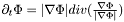
This actually creates three different channels, based on the image's x-derivative, y-derivative and cross-derivative. In LSSEG, these channels can be computed using the function compute_structure_tensor_XD(). Click here for a higher-resolution version of the below image.

An image of a zebra, with its three structure tensor components.
You can read more about the structure tensor in section 2.2 of Brox' PhD thesis.

the scale measure: (see link for definition)
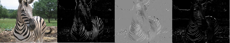
The scale measure attempts to express the size of the structures each pixel belong to, in the sense that pixels that have the same scale measure value are likely to belong to structures with the same local scale. In LSSEG, the scale measure can be computed using the function compute_scale_factor_XD(). Click here for a higher-resolution version of the below image.

An image of a zebra, with its computed scale measure (computed using 20 timesteps of duration 1)
You can read more about the scale measure in section 4.1.2 of Brox' PhD thesis.

Segmentation with multiple regions

The LSSEG library supports segmentation of a picture into more than one region. This is a complex problem, and several approaches to this exist in the literature. We have implemented an algorithm similar to what is described in section 5.3 of Brox' PhD thesis. Some characteristics of this approach are:

we use one separate level-set function for each region. This is somewhat different from the usual two-region approach, where one level-set function was sufficient to determine both regions ("inside" and "outside").
the number of regions must be specified in advance by the user.
there should be no substantial overlap between the segmented regions. For algorithmic reason, an overlap of a few pixels is tolerated.
whereas some multiregion segmentation approaches found in the literature use lagrange multipliers in order to keep different regions separate, we use a competing region approach, where the regions compete for influence along their mutual borders, and can "push" each other away.

Whereas the theoretical development can be found in section 5.3 of Brox' PhD thesis, we here aim to outline the general idea and what consequences this leads to in the LSSEG setting.

In the original evolution equation for segmentation into two regions using regional statistics, we had:

$\partial_t\Phi = |\nabla\Phi|\left[\log p_{outside} - \log p_{inside}\right] + \nu|\nabla\Phi| \left[\nabla(\frac{\nabla\Phi}{|\nabla\Phi|})\right]$

In the multi-region setting, there is no outside anymore, just a number $N$ of different competing regions described by $N$ level-set functions $\Phi_i, i=1..N$ . For a given level-set function $\Phi_i$ , we modify its evolution equation in the following way:

$\partial_t\Phi_i = |\nabla\Phi_i|\left[\log p_i + \nu div(\frac{\nabla\Phi_i}{|\nabla|Phi_i|}) - \max_{j\neq i} (\log p_j + \nu div(\frac{\nabla\Phi_j}{|\nabla\Phi_j}))\right]$

We see that the term representing the outside ( $\log p_{outside}$ ) in the original equation has now been replaced by a term $\log p_j + \nu div(\frac{\nabla\Phi_j}{|\nabla\Phi_j})$ representing the "strongest" competing candidate at the point in question. This leads to an evolution where stronger candidates "push away" weaker ones. As long as we take care to initialize the domains so that they are non-overlapping and together cover the whole image domain, this will lead to an evolution where regions stay separate while still covering the whole image domain at all times.

The multi-region setting has one important implication for the initialization of ForceGenerators when using the LSSEG library: by default the ForceGenerators NormalDistributionForce and ParzenDistributionForce compute the quantity corresponding to the normal direction flow for two-region segmentation, i.e., $(\log p_{outside} - \log p_{inside})$ . In the multi-region setting, the outside is not defined anymore, and the corresponding term, $\log p_{outside}$ must not be added to the term. For this reason, these ForceGenerators need to be told if they are going to be used in a multiregion setting. This is specified upon the construction of the ForceGenerators by a boolean argument to their constructor.

The algorithm in LSSEG that carries out the evolution of several level-set functions $\Phi_i$ in a multiresolution setting is called develop_multiregion_XD().

Note:: Multiregion segmentation is a very unstable process and its very easy to get stuck in a local minimum when looking for an optimal segmentation. In general, this segmentation is quite sensitive to the initialization. In order to obtain a good multiregion segmentation of an image with LSSEG, the user should be prepared to experiment around a bit with various settings in order to get an acceptable result.

How the parts fit together

Here, we will attempt to describe an overview of the segmentation algorithm found in the sample program called segmentation2D.

initialization of level-set functions

First of all, we define some initial partition of the image, from which to start the region development. This is carried out by a local function, initialize_levelsets(), which selects the use of one of the LSSEG functions:

sphere() (two-region segmentation - initializes the level-set function so that its inside region is a circle centered on the middle of the image)
horizontal_sinusoidal_bands() (two-region segmentation - initializes the level-set function so that its inside region becomes a set of horizontal bands across the image.
multiregion_bands() (multiregion segmentation - initializes the set of level-set functions so that their inside regions together becomes a set of horizontal bands across the image.
random_scattered_voronoi() (multiregion segmentation - initializes the set of level-set functions so that their inside regions together becomes a random, scattered partition of irregular fragments covering the image domain.

multiresolution

The first thing to mention is that we do not start a segmentation on the complete image right away. Instead, we downscale the image several times, run the segmentation on the smallest version on the image first, and then successively run the segmentation on larger versions using the previous result as an initialization. The reason for this approach is that our PDE-based segmentation approach is computationally very expensive and do not converge very rapidly on fine grids (i.e., on high-resolution images). A segmentation process with several levels off resolution allows us to converge rapidly on a coarse image, and hopefully get an initialization that is much closer to the desired result when running on higher resolutions.

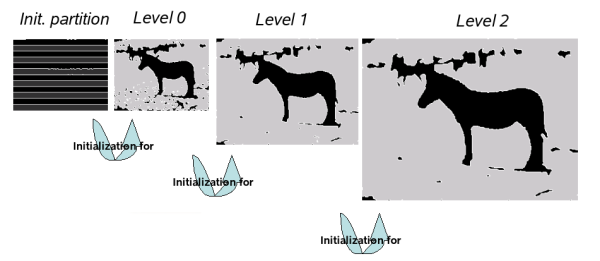
an illustration of the multilevel segmentation approach

use of an image mask

It is possible for the user to specify a Mask, which will limit the domain of the image on which the segmentation will be carried out. This can be useful in cases where only a specific part of the image is of interest for segmentation, and that the rest of the image will only "confuse" the segmentation process. A mask is an single-channeled image whose pixels are either zero (off) or nonzero (on). As such, it can be stored in any image format, as long as it is limited to a single channel.

"setting up regions"

The information needed about each region is:

the level-set function that describes its region
the scalar parameter describing the smoothness of its boundary
the ForceGenerator that determines the normal direction flow components of its evolution.

These three pieces of information are bundled together in Region objects.

assembling the information

On each level in the multiresolution process, the program assembles a "working image", whose channels contain all the information that should steer the segmentation process on that level. This may or may not include color channels, intensity channel or synthetized images ( structure tensor, scale measure) generated from the original image in order to enhance region differences. In the algorithm, this working image is called multichan in the code. The channels going into the assembly of this image can be specified by the user on the command line.

prefiltering

Before starting the segmentation process on the assembled image multichan, it is smoothed using an anisotropic smoothing process that preserves edges in the image. The benefit of this smoothing is to remove fluctuations in order for the segmentation process to converge faster and prevent getting stuck in local minima. It also distributes more evenly the information found in the structure tensor and scale measure channels. The level of smoothing to be used can be set from the command line. The user specifies a number, and when the average pixel variation between two smoothing iterations is less that that number, the smoothing process stops. For this reason, smaller numbers lead to more smoothing . In general, smoothing is good, but too much smoothing may remove important cues for the segmentation. In addition, the smoothing is computationally expensive.

call to the actual segmentation process

When the regions have been set up, and the working image (multichan) for a given level of resolution has been assembled and smoothed, the segmentation process is started. This is done through calls to the develop_single_region_2D() function or the develop_multiregion_2D() function, depending on whether we segment into two or more regions.

periodic reinitialization

With regular intervals, the segmentation process is interrupted and the level-set functions reinitialized to the signed distance function for the region they currently describe. This prevents situations where progress in the evolution of regions is "blocked" due to degenerate/extreme values in the gradient of the level-set functions. (When reinitialized to the distance function, the gradient becomes unity almost everywhere.

visualization of results

Each time the segmentation process is interrupted for reinitialization purposes, the algorithm also updates a visualization window showing the progress of the segmentation (unless told not to do so). This is done by a call to the function visualize_level_set() or visualize_multisets(), which produces images that fills the segmented region(s) with a color, and enhance the contour of the region. The produced image is then superposed on the original image and shown in the visualization window.

Below you find the segmentation result of an image of a guppy. The first segmentation contain two regions, the second contain four. The parameters for the four-region image had to be tuned more carefully. For a higher resolution image, click here.

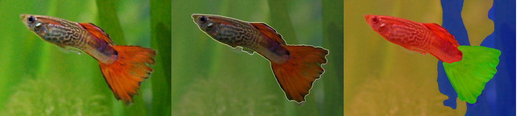
Left: original image. Center: segmented into two regions.Right: segmented into four regions

The command line for the two-regions segmentation was segmentation2D guppy.png -init 10
The command line for the four-region segmentation was segmentation2D guppy.png -init 4 -nr 4 -s 0.1 -lr 60 -i1 10000
The multi-region algorithm had to be tuned much more carefully.

Generated on Tue Nov 28 18:35:47 2006 for lsseg by

1.4.7