Multiscale Finite Volume Pressure solver: Iterative improvements

The Multiscale Finite Volume Method can be used in smoother-multiscale cycles or as a preconditioner for iterative algorithms. This example demonstrates this usage in preconditioned GMRES and Dirichlet Multiplicative / Additive Schwarz smoothing cycles.

Contents

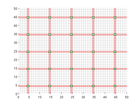
Iteration parameters

We will be doing 100 iterations in total, corresponding to 100 GMRES iterations and 10 cycles of 10 smoothings for the MsFV iterations. Omega is initially set to 1.

omega = 1;
subiter = 10;
iterations = 100;
cycles = round(iterations/subiter);

Load required modules

mrstModule add coarsegrid msfvm

Define a simple 2D Cartesian grid

We create a fine grid, and a coarse grid of $5 \times 5$ giving each coarse block fine cells. We also add geometry data to the grids.

nx = 50; ny = 50;
Nx = 5; Ny = 5;
% Instansiate the actual grid
G = cartGrid([nx, ny]);
G = computeGeometry(G);
% Generate coarse grid
p = partitionUI(G, [Nx, Ny]);
CG = generateCoarseGrid(G, p);
CG = coarsenGeometry(CG);

Dual grid

Generate the dual grid logically and plot it.

DG = partitionUIdual(CG, [Nx, Ny]);
% Plot the dual grid
clf;
plotDual(G, DG)
view(0,90), axis tight

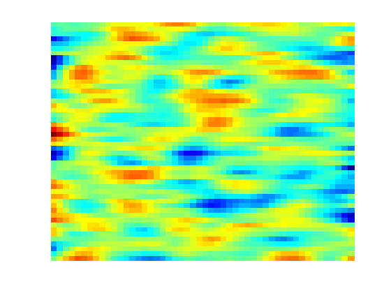
Permeability and fluid

We define a single phase fluid.

fluid        = initSingleFluid('mu' ,    1*centi*poise     , ...
                                'rho', 1014*kilogram/meter^3);
% Generate a lognormal field via porosity
poro = gaussianField(G.cartDims, [.2 .4], [11 3 3], 2.5);
K = poro.^3.*(1e-5)^2./(0.81*72*(1-poro).^2);
rock.perm    = K(:);
clf;
plotCellData(G, log10(rock.perm));
axis tight off;

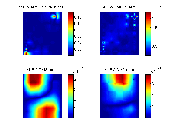
Add a simple Dirichlet boundary

bc = [];
bc = pside   (bc, G, 'LEFT', .5*barsa());
bc = pside   (bc, G, 'RIGHT', .25*barsa());

Add some wells near the corners

W = [];
cell1 = round(nx*1/8) + nx*round(ny*1/8);
cell2 = round(nx*7/8) + nx*round(ny*7/8);

W = addWell(W, G, rock, cell1,      ...
            'Type', 'bhp' , 'Val', 1*barsa(), ...
            'Radius', 0.1, 'InnerProduct', 'ip_tpf', ...
            'Comp_i', [0, 1]);

W = addWell(W, G, rock, cell2,      ...
            'Type', 'bhp' , 'Val', 0*barsa(), ...
            'Radius', 0.1, 'InnerProduct', 'ip_tpf', ...
            'Comp_i', [0, 1]);

State and tramsmissibility

Instansiate empty well and calculate transmissibility.

sol = initState(G, [], 0, [1, 0]);
T = computeTrans(G, rock);

Solve the systems

We define an anonymous function because many parameters are common to each call tol solveMSFVM_TPFA_Incomp. This makes it easy to compare different parameters without duplicating code.

solvems = @(iterations, subiterations, iterator, smoother, omega) ...
        solveMSFV_TPFA_Incomp(sol, G, CG, T, fluid, 'Wells', W, ...
        'Dual', DG, 'bc', bc,...
        'Iterations',       iterations,...
        'Subiterations',    subiterations,...
        'Iterator',         iterator,...
        'Smoother',         smoother,...
        'Omega',            omega, ...
        'Verbose',          false);

disp 'Solving reference solution';
tic; solRef = incompTPFA(sol, G, T, fluid, 'bc', bc, 'wells', W); toc;
disp 'Solving without iterations';
tic; solFV_noiter = solvems(0, 0, '', '', 0); toc;
disp 'Solving with GMRES using MsFV preconditioner';
tic; solFV_gmres = solvems(iterations, 0, 'gmres', '', 0) ;toc;
disp 'Solving with GMRES without preconditioner';
tic; solFV_direct =solvems(iterations, 0, 'gmres-direct', '', 0) ;toc;
disp 'Solving with Dirichlet Multiplicative Schwarz (DMS) smoother cycles';
tic; solFV_dms = solvems(cycles, subiter, 'msfvm', 'DMS', omega);toc;
disp 'Solving with Dirichlet Additive Schwarz (DAS) smoother cycles';
tic; solFV_das = solvems(cycles, subiter, 'msfvm', 'DAS', omega);toc;

Solving reference solution
Elapsed time is 0.011505 seconds.
Solving without iterations
Elapsed time is 0.016350 seconds.
Solving with GMRES using MsFV preconditioner
Elapsed time is 0.137220 seconds.
Solving with GMRES without preconditioner
Elapsed time is 0.161450 seconds.
Solving with Dirichlet Multiplicative Schwarz (DMS) smoother cycles
Elapsed time is 1.445621 seconds.
Solving with Dirichlet Additive Schwarz (DAS) smoother cycles
Elapsed time is 0.909103 seconds.

Plot error for the different configurations

clf;
subplot(2,2,1)
% We plot the error scaled with total variation in the reference solution.
variation = abs(max(solRef.pressure - min(solRef.pressure)));

plotCellData(G, abs(solRef.pressure - solFV_noiter.pressure) ./ variation);
view(0,90); axis tight off; colorbar;
title('MsFV error (No iterations)')
subplot(2,2,2)


plotCellData(G, abs(solRef.pressure - solFV_gmres.pressure) ./ variation);
view(0,90); axis tight off; colorbar;
title('MsFV-GMRES error')

subplot(2,2,3)
% Plot error scaled with local variation
plotCellData(G, abs(solRef.pressure - solFV_dms.pressure) ./ variation);
view(0,90); axis tight off; colorbar;
title('MsFV-DMS error')

subplot(2,2,4)
% Plot error scaled with local variation
plotCellData(G, abs(solRef.pressure - solFV_das.pressure) ./ variation);
view(0,90); axis tight off; colorbar;
title('MsFV-DAS error')

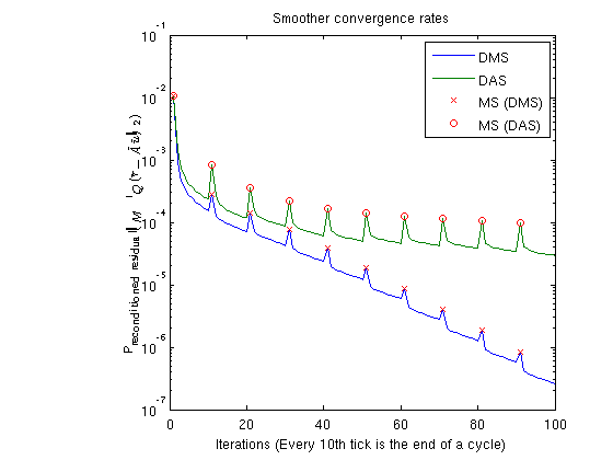
Plot smoother cycles

We plot the preconditioned residuals for the smoother cycles. Note that the residual decreases monotonically within a smoother cycle, but jumps back up when a MsFV solution is comptuted. This is because the new multiscale solution is recomptued with source terms to get a better approximation than the last smoother cycle. The end of a cycle is marked in red.

clf;

semilogy([solFV_dms.residuals; solFV_das.residuals]');
hold on
title('Smoother convergence rates');

xlabel(sprintf('Iterations (Every %dth tick is the end of a cycle)', subiter));
ylabel('Preconditioned residual($\|M^{-1}Q(\tilde{r} - \tilde{A}\tilde{u}) \|_2$)','interpreter','latex')
t_ms = 1:subiter:iterations;

semilogy(t_ms, solFV_dms.residuals(t_ms), 'rx')
semilogy(t_ms, solFV_das.residuals(t_ms), 'ro')
legend({'DMS','DAS', 'MS (DMS)', 'MS (DAS)'});

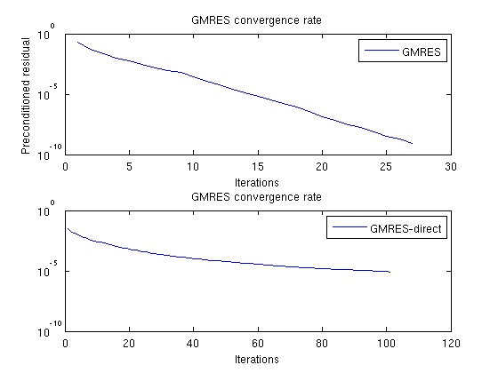
Plot residuals for GMRES

The residuals of the preconditioned GMRES are not directly comparable to GMRES without preconditioner, but we can compare the number of iterations.

clf;subplot(2,1,1)
semilogy([solFV_gmres.residuals]');
title('GMRES convergence rate'); legend({'GMRES'});
xlabel('Iterations');
ylabel('Preconditioned residual')

subplot(2,1,2);
semilogy([solFV_direct.residuals]');
title('GMRES convergence rate'); legend({'GMRES-direct'});
xlabel('Iterations');

Check error

Note that while the norms are different, the preconditioned GMRES converges while the direct GMRES does not. They both start with the same initial pressure solution. To see that the preconditioner ends up with a better result, we can compare the final pressure solutions:

disp 'With preconditioner:'
reportError(solRef.pressure, solFV_gmres.pressure);
disp 'Without preconditioner:'
reportError(solRef.pressure, solFV_direct.pressure);

With preconditioner:
ERROR:
	2: 0.00000000
	Sup: 0.00000000
	Minimum 0.00000000
Without preconditioner:
ERROR:
	2: 0.00062477
	Sup: 0.00050921
	Minimum 0.00010394