In this example we consider a synthetic sloping aquifer, created in this tutorial. The topography of the top surface and the geological layers in the model is generated by combining the membrane function (MATLAB logo) and a sinusoidal surface with random perturbations.

Here, CO₂ is injected in the aquifer for a period of 30 years. Thereafter we simulate the migration of the CO₂ in a post-injection period of 720 years.

The simulation is done using the vertical average/equilibrium framework.

Contents

Video of the simulation

Construct stratigraphic and petrophysical model

Description of how the model is created is provided in a separate tutorial.

Set time and fluid parameters

T          = 750*year();
stopInject = 30*year();
dT         = 1*year();
dTplot     = 5*dT;

% Make fluid structures, using data that are resonable at p = 300 bar
fluidVE = initVEFluid(Gt, 'mu' , [0.056641 0.30860] .* centi*poise, ...
   'rho', [686.54 975.86] .* kilogram/meter^3, ...
   'sr', 0.2, 'sw', 0.1, 'kwm', [0.2142 0.85]);
gravity on

Set well and boundary conditions

We use one well placed down the flank of the model, perforated in the bottom layer. Injection rate is 1.4e3 m^3/day of supercritical CO₂. Hydrostatic boundary conditions are specified on all outer boundaries.

% Set well in 3D model
wellIx = [G.cartDims(1:2)/5, G.cartDims([3 3])];
rate   = 2.8e3*meter^3/day;
W      = verticalWell([], G, rock, wellIx(1), wellIx(2), ...
                      wellIx(3):wellIx(4), 'Type', 'rate', 'Val', rate, ...
                      'Radius', 0.1, 'comp_i', [1,0], 'name', 'I');

% Well and BC in 2D model
wellIxVE = find(Gt.columns.cells == W(1).cells(1));
wellIxVE = find(wellIxVE - Gt.cells.columnPos >= 0, 1, 'last' );
WVE      = addWell([], Gt, rock2D, wellIxVE, ...
                   'Type', 'rate','Val',rate,'Radius',0.1);
bcVE     = addBC([], bcIxVE, 'pressure', ...
                 Gt.faces.z(bcIxVE)*fluidVE.rho(2)*norm(gravity));
bcVE     = rmfield(bcVE,'sat');
bcVE.h   = zeros(size(bcVE.face));

% for 2D/vertical average, we need to change defintion of the wells
for i=1:numel(WVE)
   WVE(i).compi = NaN;
   WVE(i).h = Gt.cells.H(WVE(i).cells);
end

Prepare simulations

Compute inner products and instantiate solution structure

SVE = computeMimeticIPVE(Gt, rock2D, 'Innerproduct','ip_simple');
preComp = initTransportVE(Gt, rock2D);
sol = initResSol(Gt, 0);
sol.wellSol = initWellSol(W, 300*barsa());
sol.h = zeros(Gt.cells.num, 1);
sol.max_h = sol.h;

Prepare plotting

We will make a composite plot that consists of several parts:

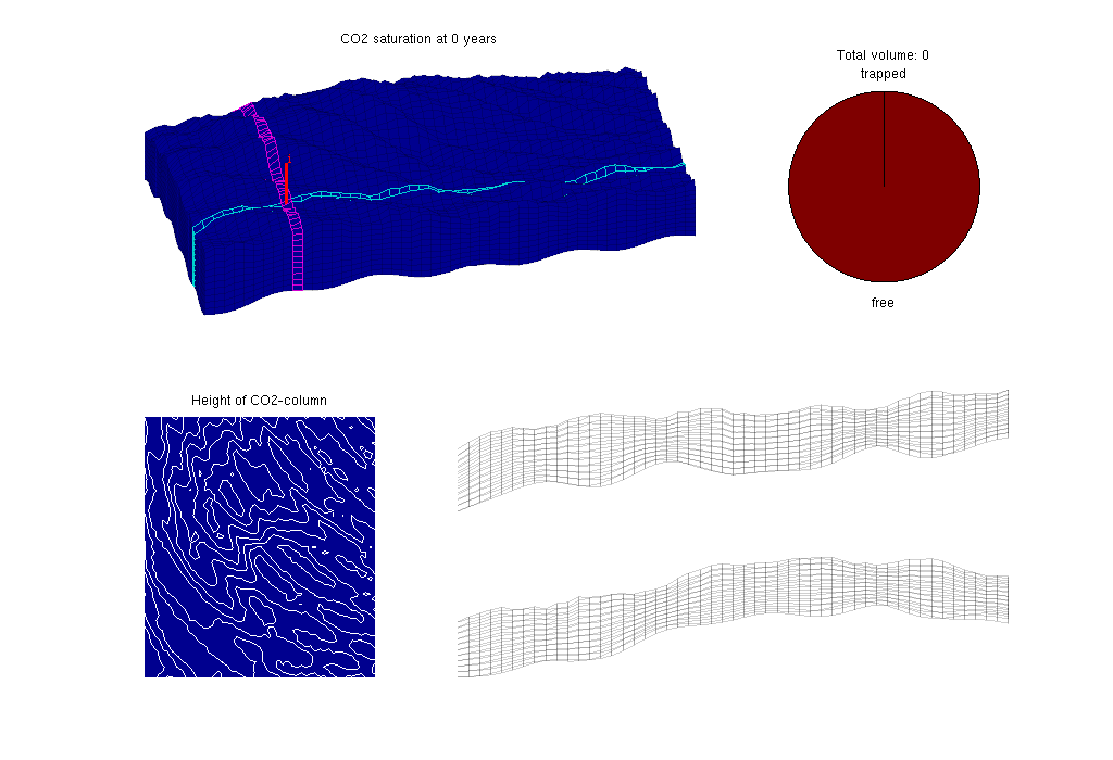
Main loop

Run the simulation using a sequential splitting with pressure and transport computed in separate steps. The transport solver is formulated with the height of the CO₂ plume as the primary unknown and the relative height (or saturation) must therefore be reconstructed.

t = 0;
while t% Advance solution: compute pressure and then transport
   sol = solveIncompFlowVE(  sol, Gt, SVE, rock, fluidVE, ...
                             'bc', bcVE, 'wells', WVE);
   sol = explicitTransportVE(sol, Gt, dT, rock, fluidVE, ...
                             'bc', bcVE, 'wells', WVE, 'preComp', preComp);

   % Reconstruct 'saturation' defined as s=h/H, where h is the height of
   % the CO2 plume and H is the total height of the formation
   sol.s = height2Sat(sol, Gt, fluidVE);
   assert( max(sol.s(:,1))<1+eps && min(sol.s(:,1))>-eps );
   t = t + dT;

   % Check if we are to stop injecting
   if t>= stopInject
      WVE  = []; bcVE = [];
   end

   % Compute trapped and free volumes of CO2
    freeVol = ...
      sum(sol.h.*rock2D.poro.*Gt.cells.volumes)*(1-fluidVE.sw);
   trappedVol = ...
      sum((sol.max_h-sol.h).*rock2D.poro.*Gt.cells.volumes)*fluidVE.sr;
   totVol = trappedVol + freeVol;

   % Plotting (...) details are provided in the full tutorial runSlopingAquifer.m accompanying the VE module. 
end

Published with MATLAB® 7.10