In this example we consider a synthetic sloping aquifier with heterogeneous petrophysical parameters that satisfy a Carman-Kozeny relation.

Contents

Top and bottom surfaces

The topography of the top surface and the geological layers in the model is generated by combining the membrane function (Matlab logo) and a sinusoidal surface with random perturbations.

clear, clc
m = 25; n = 10;
[x,y]=meshgrid(0:2*m);
T = 2 - 3*membrane(1,m) - 0.07*(x+y) - 0.3*sin(pi*x/12)*sin(pi*y/7) ...
   - 0.25*sin(pi*(x+y)/5) - 0.25*sin(pi*(x.*y)/100) - 0.3*rand(size(x));
B = 2 - 3*membrane(1,m) - 0.09*(x+y) - 0.3*sin(pi*x/15).*sin(pi*y/8) ...
   - 0.25*sin(pi*(x+y+5)/5) - 0.25*sin(pi*(x.*y)/80) + 4;
clf
mesh(x,y,T); hold on, mesh(x,y,B), hold off
set(gca,'zdir','reverse');
title('Top and bottom surface'); drawnow;

3D grid

The layers in the 3D grid are interpolated between the values of the top and bottom surfaces, before we scale and translate the whole grid to suitable dimensions.

G = tensorGrid(0:2*m,0:2*m,0:n);
num = prod(G.cartDims(1:2)+1);
for k=1:n+1
   G.nodes.coords((1:num)+(k-1)*num,3) = T(:) + (k-1)/n*(B(:)-T(:));
end
clear x y T B;
%
G.nodes.coords(:,1:2) = G.nodes.coords(:,1:2)*2e2;
G.nodes.coords(:,3) = G.nodes.coords(:,3)*15+1000;
G = computeGeometry(G);
clf
plotGrid(G); view(3), axis tight
title('3D grid'); drawnow

Top-surface grid

Make the hybrid grid structure that is uses in VE simulations and plot it slightly above the true top surface

[Gt, G] = topSurfaceGrid(G);
z = Gt.nodes.z;
Gt.nodes.z = 0.995*z;
plotGrid(Gt,'FaceColor','b');
Gt.nodes.z = z; clear z;
axis tight
title('3D grid with top surface'); drawnow

Petrophysical parameters

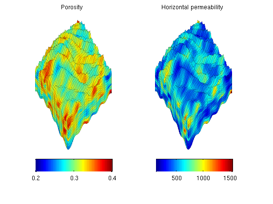
We generate porosity as a Gausiann random field and then compute the permeability using a Carman-Kozeny relationship. The permeability in the vertical direction is set to 10% of the lateral permeability.

p = gaussianField(G.cartDims, [0.2 0.4], [11 5 3], 2.5);
K = p.^3.*(1e-5)^2./(0.81*72*(1-p).^2);
rock.poro = p(G.cells.indexMap);
rock.perm = 5*K(G.cells.indexMap);
rock2D    = averageRock(rock, Gt);

clf
subplot(1,2,1),
  plotCellData(G,rock.poro,'EdgeColor','k','EdgeAlpha',0.1);
  view(3), colorbar('horiz'), axis tight off
  title('Porosity');
subplot(1,2,2);
  plotCellData(G,convertTo(rock.perm(:,1), milli*darcy),...
     'EdgeColor','k','EdgeAlpha',0.1);
  view(3), colorbar('horiz'), axis tight off
  title('Horizontal permeability');
clear p K;
drawnow

Find pressure boundary

Setting boundary conditions is unfortunately a manual process and may require some fiddling with indices, as shown in the code below. Here, we need to identify all parts of the outer boundary that are open so that we later can set an appropriate hydrostatic condition. No-flow boundaries need not be set.

% Boundary in 3D grid (works only for hexahedral grids)
i = any(G.faces.neighbors==0,2);  % find all outer faces
I = i(G.cells.faces(:,1));        % vector of all faces of all cells, true if outer
j = false(6,1);                   % mask, cells can at most have 6 faces
j(1:4)=true;                      %   extract east, west, north, south
J = j(G.cells.faces(:,2));        % vector of faces per cell, true if E,W,N,S
bcIx = G.cells.faces(I & J, 1);

clf,
subplot(2,1,1)
plotCellData(G, G.cells.centroids(:,3), ...
             'FaceAlpha', 0.5, 'EdgeColor','k', 'EdgeAlpha', 0.1)
plotFaces(G, bcIx, 'g');
view(-7,60), axis tight, title('3D grid');

% Boundary in 2D grid
i = any(Gt.faces.neighbors==0, 2);  % find all outer faces
I = i(Gt.cells.faces(:,1));         % vector of all faces of all cells, true if outer
j = false(6,1);                     % mask, cells can at most have 6 faces,
j(1:4)=true;                        %   extract east, west, north, south
J = j(Gt.cells.faces(:,2));         % vector of faces per cell, true if E,W,N,S
bcIxVE = Gt.cells.faces(I & J, 1);

subplot(2,1,2)
plotCellData(Gt, Gt.cells.z, ...
   'FaceAlpha', 0.5, 'EdgeColor','k', 'EdgeAlpha', 0.1)
plotGrid(Gt, sum(Gt.faces.neighbors(bcIxVE,:),2), 'FaceColor', 'r')
view(-7,60), axis tight, title('2D grid of top surface');

clear i j I J
drawnow

Store data

disp('    Writing SlopingAquifer.mat');
save SlopingAquifer.mat G Gt rock rock2D bcIx bcIxVE

    Writing SlopingAquifer.mat

Published with MATLAB® 7.10