Contents

Using the trapping analysis tool

In this example, we will demonstrate the use of the trapping analysis tool and a few ways to visualize and use its results. We will use the caprock of the Statfjord formation as input.

% The following line ensures that we have the necessary modules loaded
moduleCheck co2lab

Load Statfjord grid and perform spill point analysis

We first load the formation and generate the associated top surface grid using the 'getFormationTopGrid' function. Since our analysis does not have particularly high computational requirements, we do not downsample the grid.

% Loading the grid from disk
coarsening_level = 1; % grid downsampling factor (1 = no downsampling)
Gt = getFormationTopGrid('Statfjordfm', coarsening_level);

% We check the number of cells in the top surface grid.
Gt.cells.num

ans =

      122076

% We then perform the trapping analysis.
ta = trapAnalysis(Gt, false)

ta = 

           traps: [122076x1 double]
          trap_z: [116x1 double]
    trap_regions: [122076x1 double]
        trap_adj: [116x116 double]
      cell_lines: {1x116 cell}
             top: [222x1 double]

Show traps

Before doing anything else, we plot the traps on the grid in order to see their size and location. Since each trap is a discrete entity, we do not use a gradient-based colormap, but rather the Matlab 'lines' colormap, where adjacent colors are not similar.

% Top view
figure
plotCellData(Gt, ta.traps, 'edgealpha', 0.1);
view(0, 90); axis tight; colormap lines;
set(gcf, 'position', [10 10 500 800]);

% Oblique view
figure
plotCellData(Gt, ta.traps, 'edgealpha', 0.1);
view(290, 60); axis tight; colormap lines;
set(gcf, 'position', [520 10 1200 800]);

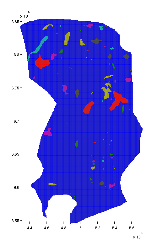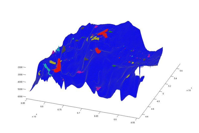Structural traps, top view	Structural traps, oblique view

Show spill regions

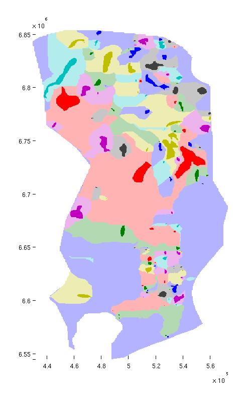
We now proceed to visualize the spill regions associated with each trap. The spill region of a trap consists of all positions in the aquifer from which CO₂ will migrate into the trap by gravity-driven migration. (By analogy with hydrology, a spill region is to a trap what a catchment area is to a lake).

Below, we plot spill regions as semi-transparent, with colors matching their associated traps.

trapfield = ta.traps;
trapfield(trapfield==0) = NaN;

% Top view
figure;
plotCellData(Gt, trapfield, 'edgecolor', 'none');
plotCellData(Gt, ta.trap_regions, 'facealpha', 0.3, 'edgecolor', 'none');
view(0, 90); axis tight; colormap lines;
set(gcf, 'position', [10 10 500 800]);

% Oblique view
figure;
plotCellData(Gt, trapfield, 'edgecolor', 'none');
plotCellData(Gt, ta.trap_regions, 'facealpha', 0.3, 'edgealpha', 0.1);
view(290, 60); axis tight; colormap lines;
set(gcf, 'position', [520 10 1200 800]);

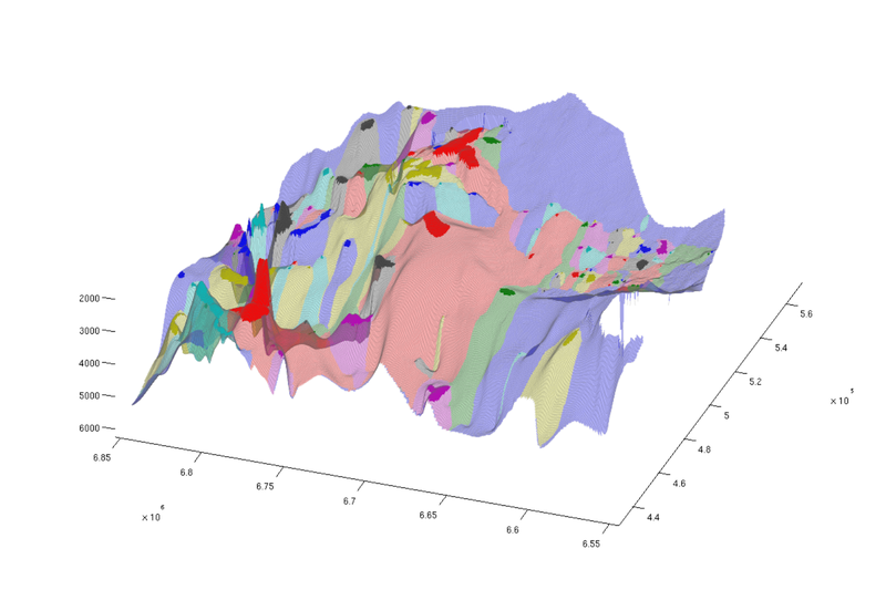Traps and spill regions, top view	Traps and spill regions, oblique view

Show size distributions in terms of area

Measured by area, there is a large spread in sizes between spill regions. The same is also the case for traps. To illustrate this point, we count the number of cells in each trap and spill region, sort them according to this size, and produce corresponding bar plots.

% We compute the number of cells in each trap region, and store the number in
% 'region_cellcount'.  This variable is thus a vector where entry 'i'
% states the number of cells belonging to trap region 'i'.
% We then produce a bar plot from the sorted result.
region_cellcount = ...
    diff(find(diff([sort(ta.trap_regions); max(ta.trap_regions)+1])));
bar(sort(region_cellcount, 'descend'));
hold on;

% We then do the same for traps.
trap_cellcount = diff(find(diff([sort(ta.traps); max(ta.traps)+1])));
bar(sort(trap_cellcount, 'descend'), 'r');

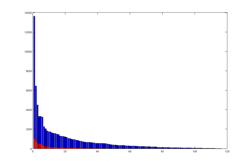Areal size distribution of spill regions (blue) and traps (red)

Each bar in these plots correspond to a trap (red) or trap region (blue), and they are sorted according to size in descending order. We can see that there is a small number of disproprtionately large traps/regions, and a long tail of very small ones.

Show the largest spill region with associated trap

We now have a closer look at the largest spill region and associated trap. To find the index of the largest spill region, we identify index of the largest entry in the vector we just constructed above. Once identified, we plot the trap and spill region in isolation.

% Find index of trap with the largest spill region
[~, ix] = max(region_cellcount);

% Visualize the trap along with the spill region
figure;
plotGrid(topSurfaceGrid(extractSubgrid(Gt.parent, find(ta.traps==ix))), ...
         'facecolor', 'r', ...
         'edgealpha', 0.1)
plotGrid(topSurfaceGrid(extractSubgrid(Gt.parent, find(ta.trap_regions==ix))), ...
         'facecolor','r', ...
         'facealpha', 0.1, ...
         'edgealpha', 0.1);
view(-64, 36);
set(gcf, 'position', [10 10 1000 700]);

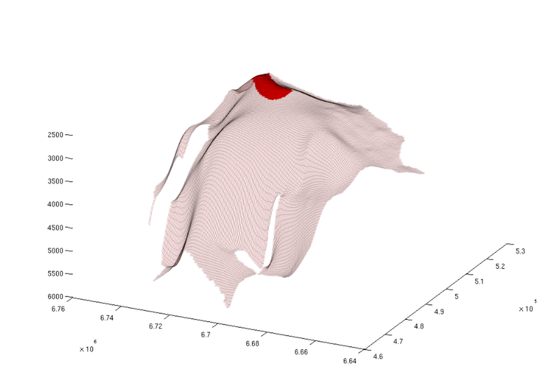Largest spill region

The plotting code above merits a word of explanation: The 'extractSubgrid' function returns a grid consisting of specified cells of the input grid. However, it does not currently work with top surface grids, so we have to provide it with the original 3D grid. Fortunately, the original grid is accessible from the top surface grid as 'Gt.parent'. Once the subgrid is produced, we generate a top surface grid from it, since that is what we wish to plot.

Show rivers

When CO₂ starts to spill out from one trap, it will migrate upwards until it hits the next. In this sense, the traps are connected in a hierarchy. We refer to the path CO₂ follows between traps as a 'river'. The cells through which these rivers run are stored in the trapping stucture, and we here use this information to produce a plot where both traps and rivers are visible.

% Identifying "river" cells
river_field = NaN(size(ta.traps));
for i = 1:numel(ta.cell_lines)
   rivers = ta.cell_lines{i};
   for r = rivers
      river_field(r{:}) = 1;
   end
end

% Producing figure with traps and rivers (top view)
figure;
plotCellData(Gt, river_field, 'edgealpha', 0.1);
plotCellData(Gt, trapfield, 'edgecolor', 'none');
view(0, 90); axis tight; colormap lines;
set(gcf, 'position', [10 10 500 800]);

% Same figure, but oblique view
figure;
plotCellData(Gt, river_field, 'edgealpha', 0.1);
plotCellData(Gt, trapfield, 'edgecolor', 'none');
view(290, 60); axis tight; colormap lines;
set(gcf, 'position', [520 10 1200 800]);

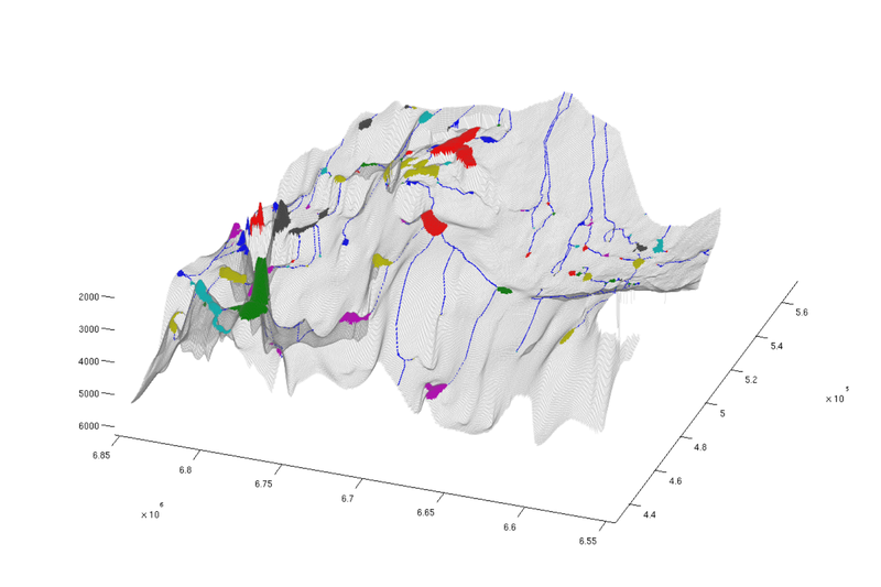Traps and rivers, top view	Traps and rivers, oblique view

Topograpical map of caprock

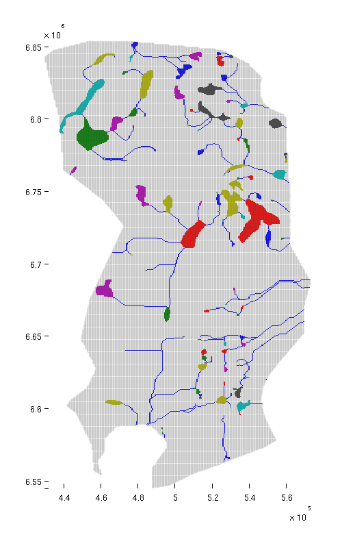
CO2lab also contains functionality for plotting topographical maps ('mapPlot'). At present, this functionality is only available as a part of the provided examples, but it can still be called from anywhere as long as the co2lab module has been loaded.

% Producing a topographical map of caprock surface, traps and rivers
h = figure;
mapPlot(h, Gt, 'traps', ta.traps, 'rivers', ta.cell_lines);
set(gcf, 'position', [10 10 500 800]);

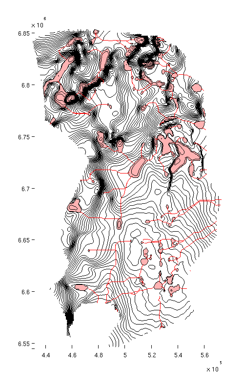Caprock with traps and rivers

Compute trap volumes

Above we have measured and sorted traps according to areal extent (i.e. number of cells). Here, we do the same thing for trap volumes. The volume of a trap can be found by adding up the volumes of its constituent cells, but only the part of that volume that is located above the trap's spill point. (The part of the cell below the spill point is not part of the trap).

In order to do this computation, we start by defining how much structural trapping volume each cell in the grid contains. For non-trap cells, this is obviously zero; for other cells it is equal to the cell's area multiplied by the vertical distance from the spill point of the trap to the top of the cell (or by the total height of the cell, whichever is smallest).

% We add a zero to the vector of spill point depths.  This is necessary for
% indexing purposes, as explained in the next comment.
depths = [0; ta.trap_z];

% The line below gives the correct "trap height" value for cells within
% traps.  For the other cells, the value is incorrect, but will be fixed by
% the succeeding line.  Note that since we have added an entry to the front
% of the 'depths' vector, we increase indices by 1.  (Otherwise, the
% presence of zeros in 'ta.traps' would cause an indexing error, since Matlab
% arrays are indexed from 1, not 0).
h = min((depths(ta.traps+1) - Gt.cells.z), Gt.cells.H);
h(ta.traps==0) = 0; % cells outside any trap should have zero trap volume

% Bulk cell volumes are now simply obtained by multiplying by the respective
% areas.  For non-trap cells, the volumes will be zero, since 'h' is zero for
% these cells.
cell_tvols = h .* Gt.cells.volumes;

% We accumulate the trap volume of individual cells to obtain the total bulk
% trap volume for each structural trap.
tvols = accumarray(ta.traps+1, cell_tvols);

% The first entry of 'tvols' contain the combined trap volume of all non-trap
% cells.  Obviously, this value should be zero, but let us check this to make
% sure.
assert(tvols(1)==0);

% We remove the first entry of 'tvols', since we are only interested in the
% volumes of the actual traps.
tvols = tvols(2:end);

% We produce a bar plot where trap volumes are plotted in descending order.
% Here too, we notice the presence of a handful of large traps, and a long
% tail of vanishingly small traps.
figure;
bar(sort(tvols, 'descend'))

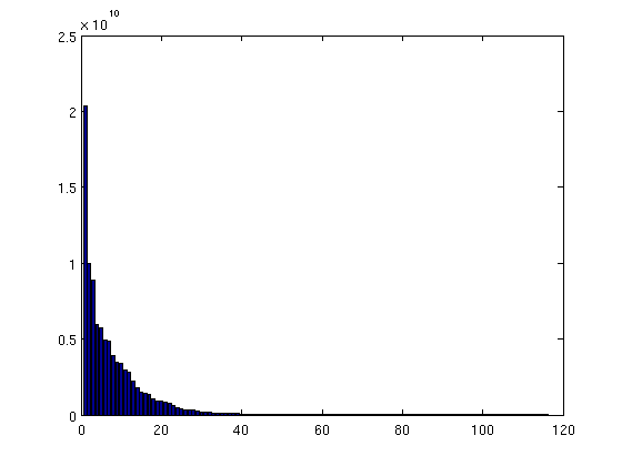Distribution of trap volumes

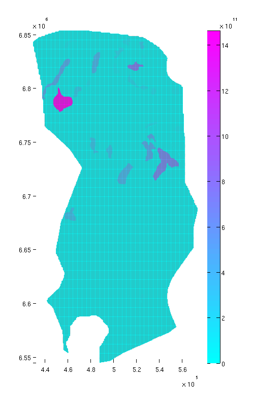
Compute and plot trap capacity in mass terms

From the purpose of CO₂ storage, it is important to be able to estimate how much CO₂ (in terms of mass) a given trap can store. This depends on its bulk volume, but also on rock porosity and local CO₂ density. (Other factors, such as residual brine saturation, also play a role, but we ignore that for now). Local CO₂ density again depends on local temperature and pressure. In order to compute CO₂ density, we therefore assume the following values:

porosity = 0.1071; % (This porosity value for Statfjord is from the Norwegian
                   % Petroleum Directorate)
seafloor_temp = 7 + 273.15; % Seafloor temperature, in degrees Kelvin
temp_grad = 30; % temperature increase per kilometer depth
rho_brine = 1000; % brine density (kilogram per cubic meter)

% Ensure that gravity is not zero
gravity on;

% computing temperature field (at caprock level)
T = seafloor_temp + temp_grad .* Gt.cells.z/1000;

% computing hydrostatic pressure (at caprock level)
P = 1 * atm + rho_brine * norm(gravity) * Gt.cells.z;

% Making stripped-down fluid object that only contains CO₂ density function
fluid = addSampledFluidProperties(struct, 'G');

% Computing local CO₂ (at caprock level)
CO2_density = fluid.rhoG(P, T);

% Computing trap capacity in mass term for each cell
cell_tmass = cell_tvols .* porosity .* CO2_density;

% Accumulating cell values to get trap capacity in mass term for each trap
tmass = accumarray(ta.traps+1, cell_tmass);
assert(tmass(1)==0);

We now plot the traps with color according to trap size.

% Normal view
figure
plotCellData(Gt, tmass(ta.traps+1), 'edgealpha', 0.1);
view(0, 90); axis tight; colormap cool; colorbar;
set(gcf, 'position', [10 10 500 800]);

% Oblique view
figure
plotCellData(Gt, tmass(ta.traps+1), 'edgealpha', 0.1);
view(290, 60); axis tight; colormap cool; colorbar;
set(gcf, 'position', [520 10 1200 800]);

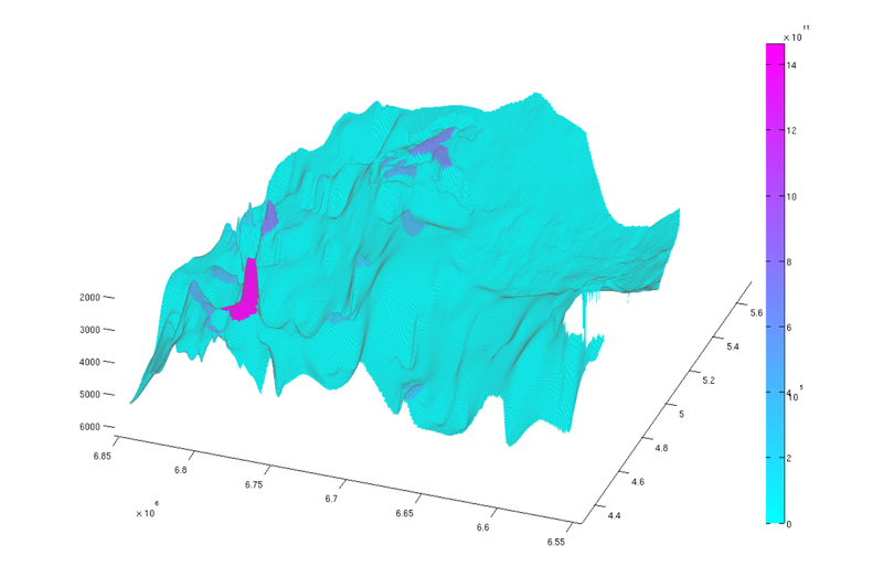Trap capacity, top view	Trap capacity, oblique view

Compute reachable structural capacity

As a final exercise, we compute the reachable structural capacity. For any given point in the aquifer, the associated reachable structural capacity is the amount of structural trapping that can be reached by gravity-driven migration from that point. This includes the capacity of the structural trap of the local spill region (if any) but also the capacity of any traps that are upstream connected to it. Naturally, traps not lying in any spill region have an associated reachable structural capcity of zero.

% We remove the first entry of 'tmass' to obtain a vector where each entry
% represents the structural capacity in mass terms of the trap with
% correspodning index. (The removed element represents the region outside any
% spill region, so it has a trapping capacity of zero).
tmass = tmass(2:end);

We compute the cumulatively reachable structural capacity by looping over all traps and adding their capacity to the grid cells that ultimately spill into it.

cum_reachable = zeros(size(ta.traps));

% Adding the capacity of each trap to its own spill region and all downstream
% regions
for trap_ix = 1:max(ta.traps)

   region = ta.trap_regions==trap_ix;

   % Counting this trap's capacity towards all cells in its spill region
   cum_reachable(region) = cum_reachable(region) + tmass(trap_ix);

   visited_regions = trap_ix;

   % Computing contribution to cells associated with downstream traps
   downstream = find(ta.trap_adj(:,trap_ix));
   while ~isempty(downstream)

      region = ta.trap_regions == downstream(1);
      cum_reachable(region) = cum_reachable(region) + tmass(trap_ix);

      visited_regions = [visited_regions;downstream(1)];

      % downstream(1) has now been processed, so we remove it from the
      % downstream vector.
      downstream = [downstream(2:end); find(ta.trap_adj(:,downstream(1)))];
      downstream = setdiff(downstream, visited_regions);
   end
end

% we divide 'cum_reachable' by 1e12 to have the result in gigatons
cum_reachable = cum_reachable / 1e12;

% Plot result (normal view)
figure
plotCellData(Gt, cum_reachable, 'edgealpha', 0.1);
view(0, 90); axis tight; colormap cool; colorbar;
set(gcf, 'position', [10 10 500 800]);

% Plot result (oblique view)
figure
plotCellData(Gt, cum_reachable, 'edgealpha', 0.1);
view(290, 60); axis tight; colormap cool; colorbar;
set(gcf, 'position', [520 10 1200 800]);

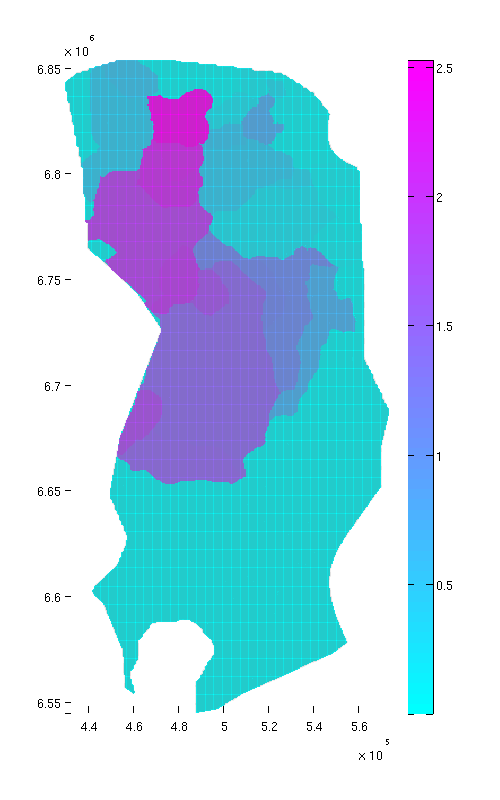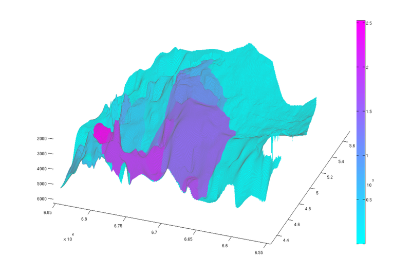Reachable struct. capacity, top view	Reachable struct. capacity, oblique view