`dual-porosity`: Dual porosity/permeability model for fractures¶

MRST’s Dual-Porosity Module¶

This module was developed by Dr. Rafael March and Victoria Spooner, of the Carbonates Reservoir Group of Heriot-Watt University (https://carbonates.hw.ac.uk/). Any inquiries, sugestions or feedback should be sent to r.march@hw.ac.uk, s.geiger@hw.ac.uk or f.doster@hw.ac.uk.

A good starting point is the single phase example in the examples folder.

Description of folders and files:

ad_models:

— DualPorosityReservoirModel: Base class for all reservoirs that show dual-porosity behaviour. — ThreePhaseBlackOilModelDP: Three-phase dual-porosity black-oil model. — TwoPhaseOilWaterModelDP: Two-phase dual-porosity oil-water model. — WaterModelDP: single-phase dual-porosity water model.

ad_modelsequations:

— equationsOilWaterDP: equations for the TwoPhaseOilWaterModelDP. — equationsWaterDP: equations for the WaterModelDP.

transfer_models:

— TransferFunction: this is a base class for all the transfer models. All the transfer models should extend this class.: The other files ending with “…TransferFunction” are special implementations of transfer functions available in the literature. The most traditional one is KazemiOilWaterGasTransferFunction (see references).

transfer_modelsshape_factor_models:

— ShapeFactor: this is a base class for all the shape factors. All the shape factors should extend this class.: The other files ending with “…ShapeFactor” are special implementations of shape factors available in the literature. The most traditional one is KazemiShapeFactor (see references).

examples:

— example_1ph: oil production by depletion in a dual-porosity reservoir. — example_2ph_imbibition: water injection and oil production by imbibition in a dual-porosity reservoir.

References: [1] Kazemi et al. Numerical Simulation of Water-Oil Flow in Naturally Fractured Reservoirs, SPE Journal, 1976 [2] Quandalle and Sabathier. Typical Features of a Multipurpose Reservoir Simulator, SPE Journal, 1989 [3] Lu et al. General Transfer Functions for Multiphase Flow in Fractured Reservoirs, SPE Journal, 2008

class DualPorosityReservoirModel(G, varargin)¶

Base class for physical models

Synopsis:

model = ReservoirModel(G, rock, fluid)

Description:

Extension of PhysicalModel class to accomodate reservoir-specific features such as fluid and rock as well as commonly used phases and variables.

Keyword Arguments:
Parameters:	G – Simulation grid. rock – Valid rock used for the model. fluid – Fluid model used for the model.
	‘property’ – Set property to the specified value.
Returns:	Class instance.

See also

ThreePhaseBlackOilModel, TwoPhaseOilWaterModel, PhysicalModel

addBoundaryConditionsAndSources(model, eqs, names, types, state, p, s, mob, rho, dissolved, components, forces)¶

Add in the boundary conditions and source terms to equations

Synopsis:

[eqs, state] = addBoundaryConditionsAndSources(model, eqs, names, types, state, ...
                                                     p, sat, mob, rho, ...
                                                     rs, components, ...
                                                     drivingForces);

Parameters:

model – Class instance.
eqs – Cell array of equations that are to be updated.
names – The names of the equations to be updated. If phase-pseudocomponents are to be used, the names must correspond to some combination of “water”, “oil”, “gas” if no special component treatment is to be introduced.
types – Cell array with the types of “eqs”. Note that these types must be ‘cell’ where source terms is to be added.
src – Struct containing all the different source terms that were computed and added to the equations.
p – Cell array of phase pressures.
s – Cell array of phase saturations.
mob – Cell array of phase mobilities
rho – Cell array of phase densities
dissolved – Cell array of dissolved components for black-oil style pseudocompositional models.
components – Cell array of equal length to the number of components. The exact representation may vary based on the model, but the respective sub-component is passed onto addComponentContributions.
forces – DrivingForces struct (see getValidDrivingForces) containing (possibily empty) src and bc fields.

Returns:

eqs – Equations with corresponding source terms added.
state – Reservoir state. Can be modified to store e.g. boundary fluxes due to boundary conditions.
src – Normalized struct containing the source terms used.

Note

This function accomodates both the option of black-oil pseudocomponents (if the model equations are named “oil”, “gas” or water) and true components existing in multiple phases. Mixing the two behaviors can lead to unexpected source terms.

addComponentContributions(model, cname, eq, component, src, force)¶

For a given component conservation equation, compute and add in source terms for a specific source/bc where the fluxes have already been computed.

Parameters:

model – (Base class, automatic)
cname – Name of the component. Must be a property known to the model itself through getProp and getVariableField.
eq – Equation where the source terms are to be added. Should be one value per cell in the simulation grid (model.G) so that the src.sourceCells is meaningful.
component – Cell-wise values of the component in question. Used for outflow source terms only.
src – Source struct containing fields for fluxes etc. Should be constructed from force and the current reservoir state by computeSourcesAndBoundaryConditionsAD.
force – Force struct used to produce src. Should contain the field defining the component in question, so that the inflow of the component through the boundary condition or source terms can accurately by estimated.

static adjustStepFromSatBounds(s, ds)¶: Ensure that cellwise increment for each phase is done with the same length, in a manner that avoids saturation violations.

compVarIndex(model, name)¶

Find the index of a component variable by name

Synopsis:

index = model.compVarIndex('co2')

Parameters:	model – Class instance name – Name of component.
Returns:	index – Index of the component for this model. Empty if saturation was not known to model.

evaluateRelPerm(model, sat, varargin)¶

Evaluate relative permeability corresponding to active phases

Synopsis:

% Single-phase water model
krW = model.evaluateRelPerm({sW});
% Two-phase oil-water model
[krW, krO] = model.evaluateRelPerm({sW, sO});
% Two-phase water-gas model
[krW, krG] = model.evaluateRelPerm({sW, sG});
% Three-phase oil-water-gas model
[krW, krO, krG] = model.evaluateRelPerm({sW, sO, sG});

Parameters:	model – The model sat – Cell array containing the saturations for all active phases.
Returns:	varargout – One output argument per phase present, corresponding to evaluated relative permeability functions for each phase in the canonical ordering.

See also

relPermWOG, relPermWO, relPermOG, relPermWG

getActivePhases(model)¶

Get active flag for MRST’s canonical phase ordering (WOG)

Synopsis:

[act, indices] = model.getActivePhases();

Parameters:	model – Class instance
Returns:	isActive – Total number of known phases array with booleans indicating if that phase is present. MRST uses a ordering of water, oil and then gas. phInd – Indices of the phases present. For instance, if water and gas are the only ones present, `phInd = [1, 3]`

getComponentNames(model)¶

#ok Get the names of components for the model .. rubric:: Synopsis:

names = model.getComponentNames();

Parameters:	model – Class instance.
Returns:	names – Cell array of component names in no particular order.

getConvergenceValues(model, problem, varargin)¶: Check convergence criterion. Relies on FacilityModel to check wells.

See also

ad_core.models.PhysicalModel.checkConvergence

getExtraWellContributions(model, well, wellSol0, wellSol, q_s, bh, packed, qMass, qVol, dt, iteration)¶

This function is called by the well model (base class: SimpleWell) during the assembly of well equations and addition of well source terms. The purpose of this function, given the internal variables of the well model, is to compute the additional closure equations and source terms that the model requires. For instance, if the model contains different components that require special treatment (see for example the implementation of this function in ad_eor.models.OilWaterPolymerModel in the ad-eor module), this function should assemble any additional equations and corresponding source terms. It is also possible to add source terms without actually adding well equations.

Returns:

compEqs – A cell array of additional equations added to the system to account for the treatment of components etc in the well system.
compSrc – Cell array of component source terms, ordered and with the same length as the output from ReservoirModel.getComponentNames.
eqNames – Names of the added equations. Must correspond to the same entries as getExtraWellEquationNames (but does not have to maintain the same ordering).

Note

Input arguments are intentionally undocumented and subject to change. Please see SimpleWell for details.

getExtraWellEquationNames(model)¶

Get the names and types of extra well equations in model

Synopsis:

[names, types] = model.getExtraWellEquationNames();

Parameters:	model – Base class.
Returns:	names – Cell array of additional well equations. types – Cell array of corresponding types to `names`.

See also

getExtraWellContributions

getExtraWellPrimaryVariableNames(model)¶

Get the names of extra well primary variables required by model.

Synopsis:

names = model.getExtraWellPrimaryVariableNames();

Parameters:	model – Class instance
Returns:	names – Cell array of named primary variables.

See also

getExtraWellContributions

getGravityGradient(model)¶

Get the discretized gravity contribution on faces

Synopsis:

gdz = model.getGravityGradient();

Parameters:	model – Class instance
Returns:	g – One entry of the gravity contribution per face in the grid. Does not necessarily assume that gravity is aligned with one specific direction.

See also

gravity

getGravityVector(model)¶

Get the gravity vector used to instantiate the model

Synopsis:

g = model.getGravityVector();

Parameters:	model – Class instance
Returns:	g – `model.G.griddim` long vector representing the gravity accleration constant along increasing depth.

See also

gravity

getMaximumTimestep(model, state, state0, dt, drivingForces)¶: Define the maximum allowable time-step based on physics or discretization choice

getPhaseIndex(model, phasename)¶

Query the index of a phase in the model’s ordering

Synopsis:

index = model.getPhaseNames();

Parameters:	model – Class instance phasename – The name of the phase to be found.
Returns:	index – Index of phase `phasename`

getPhaseIndices(model)¶: Get the active phases in canonical ordering

getPhaseNames(model)¶

Get short and long names of the present phases.

Synopsis:

[phNames, longNames] = model.getPhaseNames();

Parameters:	model – Class instance
Returns:	phNames – Cell array containing the short hanes (‘W’, ‘O’, G’) of the phases present longNames – Longer names (‘water’, ‘oil’, ‘gas’) of the phases present.

getScalingFactorsCPR(model, problem, names, solver)¶

#ok Get scaling factors for CPR reduction in CPRSolverAD

Parameters:	model – Class instance problem – `LinearizedProblemAD` which is intended for CPR preconditioning. names – The names of the equations for which the factors are to be obtained. solver – The `LinearSolverAD` class requesting the scaling factors.
Returns:	scaling – Cell array with either a scalar scaling factor for each equation, or a vector of equal length to that equation.

SEE ALSO: CPRSolverAD

getSurfaceDensities(model)¶

Get the surface densities of the active phases in canonical ordering (WOG, with any inactive phases removed).

Returns:	rhoS – pvt x n double array of surface densities.

getValidDrivingForces(model)¶: Get valid forces. This class adds support for wells, bc and src.

See also

ad_core.models.PhysicalModel.getValidDrivingForces

getVariableField(model, name, varargin)¶

Map variables to state field.

Dual porosity: variable names

insertWellEquations(model, eqs, names, types, wellSol0, wellSol, wellVars, wellMap, p, mob, rho, dissolved, components, dt, opt)¶

Add in the effect of wells to a system of equations, by adding corresponding source terms and augmenting the system with additional equations for the wells.

Parameters:

eqs – Cell array of equations that are to be updated.
names – The names of the equations to be updated. If phase-pseudocomponents are to be used, the names must correspond to some combination of “water”, “oil”, “gas” if no special component treatment is to be introduced.
types – Cell array with the types of “eqs”. Note that these types must be ‘cell’ where source terms is to be added.
src – Struct containing all the different source terms that were computed and added to the equations.
various – Additional input arguments correspond to standard reservoir-well coupling found in `FacilityModel.

static relPermOG(so, sg, f, varargin)¶

Two-phase oil-gas relative permeability function

Synopsis:

[krO, krG] = model.relPermOG(so, sg, f);

Parameters:	sw – Water saturation sg – Gas saturation f – Struct representing the field. Fields that are used: `krO`: Oil relperm function of oil saturation. `krOG`: Oil-gas relperm function of gas saturation. This function is only used if `krO` is not found. `krG`: Gas relperm function of gas saturation.
Returns:	krO – Oil relative permeability. krG – Gas relative permeability

Note

This function should typically not be called directly as its interface is subject to change. Instead, use evaluateRelPerm.

static relPermWG(sw, sg, f, varargin)¶

Two-phase water-gas relative permeability function

Synopsis:

[krW, krG] = model.relPermWG(sw, sg, f);

Parameters:	sw – Water saturation sg – Gas saturation f – Struct representing the field. Fields that are used: `krW`: Water relperm function of water saturation. `krG`: Gas relperm function of gas saturation.
Returns:	krW – Water relative permeability. krG – Gas relative permeability

Note

This function should typically not be called directly as its interface is subject to change. Instead, use evaluateRelPerm.

static relPermWO(sw, so, f, varargin)¶

Two-phase water-oil relative permeability function

Synopsis:

[krW, krO] = model.relPermWO(sw, so, f);

Parameters:	sw – Water saturation so – Oil saturation f – Struct representing the field. Fields that are used: `krW`: Water relperm function of water saturation. `krO`: Oil relperm function of oil saturation. `krOW`: Oil-water relperm function of oil saturation. Only used if `krO` is not found.
Returns:	krW – Water relative permeability. krO – Oil relative permeability.

Note

This function should typically not be called directly as its interface is subject to change. Instead, use evaluateRelPerm.

static relPermWOG(sw, so, sg, f, varargin)¶

Three-phase water-oil-gas relative permeability function

Synopsis:

[krW, krO, krG] = model.relPermWOG(sw, so, sg, f);

Parameters:	sw – Water saturation so – Oil saturation sg – Gas saturation f – Struct representing the field. Fields that are used: `krW`: Water relperm function of water saturation. `krOW`: Oil-water relperm function of oil saturation. `krOG`: Oil-gas relperm function of oil saturation. `krG`: Gas relperm function of gas saturation. `sWcon`: Connate water saturation. OPTIONAL.
Returns:	krW – Water relative permeability. krO – Oil relative permeability. krG – Gas relative permeability

Note

This function should typically not be called directly as its interface is subject to change. Instead, use evaluateRelPerm.

satVarIndex(model, name)¶

Find the index of a saturation variable by name

Synopsis:

index = model.satVarIndex('water')

Parameters:	model – Class instance name – Name of phase.
Returns:	index – Index of the phase for this model. Empty if saturation was not found.

satVarIndexMatrix(model, name)¶

Find the index of a saturation variable by name

Synopsis:

index = model.satVarIndex('water')

Parameters:	model – Class instance name – Name of phase.
Returns:	index – Index of the phase for this model. Empty if saturation was not found.

setPhaseData(model, state, data, fld, subs)¶

Store phase data in state for further output.

Synopsis:

state = model.setPhaseData(state, data, 'someField')
state = model.setPhaseData(state, data, 'someField', indices)

Description:

Utility function for storing phase data in the state. This is used for densities, fluxes, mobilities and so on when requested from the simulator.

Parameters:	model – Class instance data – Cell array of data to be stored. One entry per active phase in `model`. fld – The field to be stored. subs – OPTIONAL. The subset for which phase data is to be stored. Must be a valid index of the type data.(fld)(subs, someIndex) = data{i} for all i. Defaults to all indices.
Returns:	state – state with updated `fld`.

setupOperators(model, G, rock, varargin)¶

Set up default discretization operators and other static props

Synopsis:

model = model.setupOperators(G, rock)

Description:

This function calls the default set of discrete operators as implemented by setupOperatorsTPFA. The default operators use standard choices for reservoir simulation similar to what is found in commercial simulators: Single-point potential upwind and two-point flux approximation.

Parameters:	model – Class instance. G – The grid used for computing the operators. Must have geometry information added (typically from `computeGeometry`). Although this is a property on the model, we allow for passing of a different grid for the operator setup since this is useful in some workflows. rock – Rock structure. See `makeRock`.
Returns:	model – Model with updated `operators` property.

Note

This function is called automatically during class construction.

splitPrimaryVariables(model, vars)¶

Split cell array of primary variables into grouping .. rubric:: Synopsis:

[restVars, satVars, wellVars] = model.splitPrimaryVariables(vars)

Description:

Split a set of primary variables into three groups: Well variables, saturation variables and the rest. This is useful because the saturation variables usually are updated together, and the well variables are a special case.

Parameters:	model – Class instance. vars – Cell array with names of primary variables
Returns:	restVars – Names of variables that are not saturations or belong to the wells. satVars – Names of the saturation variables present in `vars`. wellVars – Names of the well variables present in `vars`

storeBoundaryFluxes(model, state, qW, qO, qG, forces)¶

Store integrated phase fluxes on boundary in state.

Synopsis:

Three-phase case
state = model.storeBoundaryFluxes(state, vW, vO, vG, forces);
% Only water and gas in model:
state = model.storeBoundaryFluxes(state, vW, [], vG, forces);

Parameters:	model – Class instance vW – Water fluxes, one value per BC interface. vO – Oil fluxes, one value per BC interface. vG – Gas fluxes, one value per BC interface. forces – `drivingForces` struct containing any boundary conditions used to obtain fluxes.
Returns:	state – State with stored values

See also

storeFluxes

storeDensity(model, state, rhoW, rhoO, rhoG)¶

Store phase densities per-cell in state.

Synopsis:

Three-phase case
state = model.storeDensity(state, rhoW, rhoO, rhoG);
% Only water and gas in model:
state = model.storeDensity(state, rhoW, [], rhoG);

Parameters:	model – Class instance rhoW – Water densities, one value per internal interface. rhoO – Oil densities, one value per internal interface. rhoG – Gas densities, one value per internal interface.
Returns:	state – State with stored values

See also

storeMobilities

storeFluxes(model, state, vW, vO, vG)¶

Store integrated internal phase fluxes in state.

Synopsis:

Three-phase case
state = model.storeFluxes(state, vW, vO, vG);
% Only water and gas in model:
state = model.storeFluxes(state, vW, [], vG);

Parameters:	model – Class instance vW – Water fluxes, one value per internal interface. vO – Oil fluxes, one value per internal interface. vG – Gas fluxes, one value per internal interface.
Returns:	state – State with stored values

See also

storeBoundaryFluxes

storeMobilities(model, state, mobW, mobO, mobG)¶

Store phase mobility per-cell in state.

Synopsis:

Three-phase case
state = model.storebfactors(state, mobW, mobO, mobG);
% Only water and gas in model:
state = model.storebfactors(state, mobW, [], mobG);

Parameters:	model – Class instance mobW – Water mobilities, one value per internal interface. mobO – Oil mobilities, one value per internal interface. mobG – Gas mobilities, one value per internal interface.
Returns:	state – State with stored values

See also

storeMobilities

storeUpstreamIndices(model, state, upcw, upco, upcg)¶

Store upstream indices for each phase in state.

Synopsis:

Three-phase case
state = model.storeUpstreamIndices(state, upcw, upco, upcg);
% Only water and gas in model:
state = model.storeUpstreamIndices(state, upcw, [], upcg);

Parameters:	model – Class instance upcw – Water upwind indicator, one value per internal interface. upco – Oil upwind indicator, one value per internal interface. upcg – Gas upwind indicator, one value per internal interface.
Returns:	state – State with stored values

See also

storeBoundaryFluxes, storeFluxes

storebfactors(model, state, bW, bO, bG)¶

Store phase reciprocal FVF per-cell in state.

Synopsis:

Three-phase case
state = model.storebfactors(state, bW, bO, bG);
% Only water and gas in model:
state = model.storebfactors(state, bW, [], bG);

Parameters:	model – Class instance bW – Water reciprocal FVF, one value per internal interface. bO – Oil reciprocal FVF, one value per internal interface. bG – Gas reciprocal FVF, one value per internal interface.
Returns:	state – State with stored values

See also

storeDensities

updateAfterConvergence(model, state0, state, dt, drivingForces)¶: Generic update function for reservoir models containing wells.

See also

ad_core.models.PhysicalModel.updateAfterConvergence

updateForChangedControls(model, state, forces)¶: Called whenever controls change.

Note

The addition this class makes is also updating the well solution and the underlying FacilityModel class instance.

See also

ad_core.models.PhysicalModel.updateForChangedControls

updateSaturations(model, state, dx, problem, satVars)¶

Update of phase-saturations

Synopsis:

state = model.updateSaturations(state, dx, problem, satVars)

Description:

Update saturations (likely state.s) under the constraint that the sum of volume fractions is always equal to 1. This assumes that we have solved for n - 1 phases when n phases are present.

Parameters:	model – Class instance state – State to be updated dx – Cell array of increments, some of which correspond to saturations problem – `LinearizedProblemAD` class instance from which `dx` was obtained. satVars – Cell array with the names of the saturation variables.
Returns:	state – Updated state with saturations within physical constraints.

See also

splitPrimaryVariables

updateSaturationsMatrix(model, state, dx, problem, satMatrixVars)¶

Update of phase-saturations

Synopsis:

state = model.updateSaturations(state, dx, problem, satVars)

Description:

Update saturations (likely state.s) under the constraint that the sum of volume fractions is always equal to 1. This assumes that we have solved for n - 1 phases when n phases are present.

Parameters:	model – Class instance state – State to be updated dx – Cell array of increments, some of which correspond to saturations problem – `LinearizedProblemAD` class instance from which `dx` was obtained. satVars – Cell array with the names of the saturation variables.
Returns:	state – Updated state with saturations within physical constraints.

See also

splitPrimaryVariables

updateState(model, state, problem, dx, drivingForces)¶: Generic update function for reservoir models containing wells.

See also

ad_core.models.PhysicalModel.updateState

validateModel(model, varargin)¶: Validate model.

See also

ad_core.models.PhysicalModel.validateModel

validateState(model, state)¶: Validate initial state.

See also

ad_core.models.PhysicalModel.validateState

FacilityModel = None¶: Facility model used to represent wells

FlowPropertyFunctions = None¶: Grouping for flow properties

FluxDiscretization = None¶: Grouping for flux discretization

dpMaxAbs = None¶: Maximum absolute pressure change

dpMaxRel = None¶: Maximum relative pressure change

dsMaxAbs = None¶: Maximum absolute saturation change

extraStateOutput = None¶: Write extra data to states. Depends on submodel type.

extraWellSolOutput = None¶: Output extra data to wellSols: GOR, WOR, …

fluid = None¶: The fluid model. See initSimpleADIFluid, initDeckADIFluid

gas = None¶: Indicator showing if the vapor/gas phase is present

gravity = None¶: Vector for the gravitational force

inputdata = None¶: Input data used to instantiate the model

maximumPressure = None¶: Maximum pressure allowed in reservoir

minimumPressure = None¶: Minimum pressure allowed in reservoir

oil = None¶: Indicator showing if the liquid/oil phase is present

outputFluxes = None¶: Store integrated fluxes in state.

rock = None¶: The rock structure (perm/poro/ntg). See makeRock.

useCNVConvergence = None¶: Use volume-scaled tolerance scheme

water = None¶: Indicator showing if the aqueous/water phase is present

class ThreePhaseBlackOilModelDP(G, rock, fluid, varargin)¶

Three phase with optional dissolved gas and vaporized oil

getPrimaryVariables(model, state)¶: Get primary variables from state, before a possible initialization as AD.

getScalingFactorsCPR(model, problem, names, solver)¶: Get approximate, impes-like pressure scaling factors

validateModel(model, varargin)¶: Validate model.

See also

ad_core.models.PhysicalModel.validateModel

validateState(model, state)¶: Check parent class

disgas = None¶: Flag deciding if oil can be vaporized into the gas phase

drsMaxRel = None¶: Maximum absolute Rs/Rv increment

vapoil = None¶: Maximum relative Rs/Rv increment

class TwoPhaseOilWaterModelDP(G, rock, fluid, varargin)¶: Two phase oil/water system without dissolution

class WaterModelDP(G, rock, fluid, varargin)¶: Single phase water model.

equationsOilWaterDP(state0, state, model, dt, drivingForces, varargin)¶

Generate linearized problem for the two-phase oil-water model

Synopsis:

[problem, state] = equationsOilWater(state0, state, model, dt, drivingForces)

Description:

This is the core function of the two-phase oil-water solver. This function assembles the residual equations for the conservation of water and oil as well as required well equations. By default, Jacobians are also provided by the use of automatic differentiation.

Keyword Arguments:
Parameters:	state0 – Reservoir state at the previous timestep. Assumed to have physically reasonable values. state – State at the current nonlinear iteration. The values do not need to be physically reasonable. model – TwoPhaseOilWaterModel-derived class. Typically, equationsOilWater will be called from the class getEquations member function. dt – Scalar timestep in seconds. drivingForces – Struct with fields: * W for wells. Can be empty for no wells. * bc for boundary conditions. Can be empty for no bc. * src for source terms. Can be empty for no sources.
	‘Verbose’ – Extra output if requested. ‘reverseMode’ – Boolean indicating if we are in reverse mode, i.e. solving the adjoint equations. Defaults to false. ‘resOnly’ – Only assemble residual equations, do not assemble the Jacobians. Can save some assembly time if only the values are required. ‘iterations’ – Nonlinear iteration number. Special logic happens in the wells if it is the first iteration.
Returns:	problem – LinearizedProblemAD class instance, containing the water and oil conservation equations, as well as well equations specified by the WellModel class. state – Updated state. Primarily returned to handle changing well controls from the well model.

See also

equationsBlackOil, TwoPhaseOilWaterModel

equationsWaterDP(state0, state, model, dt, drivingForces, varargin)¶

Generate linearized problem for the single-phase water model

Synopsis:

[problem, state] = equationsWater(state0, state, model, dt, drivingForces)

Description:

This is the core function of the single-phase water solver with black-oil style properties. This function assembles the residual equations for the conservation of water and oil as well as required well equations. By default, Jacobians are also provided by the use of automatic differentiation.

Keyword Arguments:
Parameters:	state0 – Reservoir state at the previous timestep. Assumed to have physically reasonable values. state – State at the current nonlinear iteration. The values do not need to be physically reasonable. model – WaterModel-derived class. Typically, equationsWater will be called from the class getEquations member function. dt – Scalar timestep in seconds. drivingForces – Struct with fields: * W for wells. Can be empty for no wells. * bc for boundary conditions. Can be empty for no bc. * src for source terms. Can be empty for no sources.
	‘Verbose’ – Extra output if requested. ‘reverseMode’ – Boolean indicating if we are in reverse mode, i.e. solving the adjoint equations. Defaults to false. ‘resOnly’ – Only assemble residual equations, do not assemble the Jacobians. Can save some assembly time if only the values are required. ‘iterations’ – Nonlinear iteration number. Special logic happens in the wells if it is the first iteration.
Returns:	problem – LinearizedProblemAD class instance, containing the equation for the water pressure, as well as well equations specified by the WellModel class. state – Updated state. Primarily returned to handle changing well controls from the well model.

See also

equationsBlackOil, ThreePhaseBlackOilModel

class EclipseTwoPhaseTransferFunction(shape_factor_name, block_dimension)¶

This is the transfer function defined in Eclipse simulator. This is a two-phase version.

calculate_transfer(ktf, model, fracture_fields, matrix_fields)¶: All calculate_transfer method should have this call. This is a “sanity check” that ensures that the correct structures are being sent to calculate the transfer

validate_fracture_matrix_structures(ktf, fracture_fields, matrix_fields)¶: We use the superclass to validate the structures of matrix/fracture variables

class TransferFunction¶

TRANSFERFN Summary of this class goes here: Detailed explanation goes here

Description:

Base Transfer function class

calculate_transfer(tf, model, fracture_fields, matrix_fields)¶: This method should be reimplemented in the derived classes

class CoatsShapeFactor(block_dimension)¶

Coats_SHAPE_FACTOR

calculates the shape factor handling anisotropic permeability dimensions are k.L^-2 when the permeability is isotropic this formula collapses to km.sigma as quoted in the literature

class ConstantShapeFactor(block_dimension, shape_factor_value)¶

CONSTANT SHAPE FACTOR

class to provide a constant given shape factor

class KazemiShapeFactor(block_dimension)¶

KAZEMI_SHAPE_FACTOR

calculates the shape factor handling anisotropic permeability dimensions are k.L^-2 when the permeability is isotropic this formula collapses to km.sigma as quoted in the literature

class LimAzizShapeFactor(block_dimension)¶

Lim and Aziz_SHAPE_FACTOR

calculates the shape factor handling anisotropic permeability dimensions are k.L^-2 when the permeability is isotropic this formula collapses to km.sigma as quoted in the literature

class ShapeFactor(block_dimension)¶

SHAPE_FACTOR Summary of this class goes here: Detailed explanation goes here

PROPERTIES lx,ly,lz are the dimensions of the matrix block

these are claculated as the inverse of the fracture spacing provided by the user

class WarrenRootShapeFactor(block_dimension)¶

WARRENANDROOT_SHAPE_FACTOR

calculates the shape factor handling anisotropic permeability dimensions are k.L^-2 when the permeability is isotropic this formula collapses to km.sigma as quoted in the literature

Warren and Root 1963: sigma = 4n(n+1)/l^2 where n is the sets of normal fractures here n is assumed to be 1

Examples¶

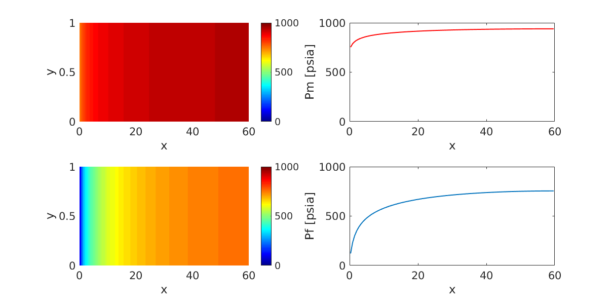
Single-phase depletion of a dual-porosity reservoir. Fracture fluid is¶

Generated from example_1ph.m

produced before the matrix. Note that the pressure drop is faster in the fractures, while the matrix drains slowly.

clear;
clc;
close all;

mrstModule add ad-blackoil ad-core ad-props dual-porosity

Set up grid¶

G = cartGrid([100, 1, 1], [60, 1, 1]*meter);
G = computeGeometry(G);

Set up rock properties¶

rock_matrix = makeRock(G, 1*darcy, .3);
rock_fracture = makeRock(G, 1000*darcy, .01);

Set up fluid¶

fluid_matrix = initSimpleADIFluid('phases', 'W', 'c', 1e-06);
fluid_fracture = initSimpleADIFluid('phases', 'W', 'c', 1e-06);

Set the DP model. Here, a single-phase model is used. Rock and fluid¶

are sent in the constructor as a cell array {fracture,matrix}

model = WaterModelDP(G, {rock_fracture,rock_matrix},...
                        {fluid_fracture,fluid_matrix});

Setting transfer function. This step is important to ensure that fluids¶

will be transferred from fracture to matrix (and vice-versa). There are several options of shape factor (see folder transfer_models/shape_factor_models/) that could be set in this constructor. The second argument is the matrix block size.

model.transfer_model_object = KazemiSinglePhaseTransferFunction('KazemiShapeFactor',...
                                                                [10,10,10]);

Initializing state¶

state = initResSol(G, 1000*psia);
state.wellSol = initWellSolAD([], model, state);
state.pressure_matrix = state.pressure;

Boundary conditions¶

bc = pside([], G, 'xmin', 0*psia, 'sat', 1);

Solver¶

solver = NonLinearSolver();

Validating model¶

model = model.validateModel();

Figure¶

fig1 = figure('Position',[100,100,1200,600]);
fig1.Color = 'w';
colormap('jet');

Time loop¶

dt = 0.1*day;
tmax = 100*dt;
t = 0;
while t<=tmax

    disp(['Time = ',num2str(t/day), ' days'])
    state = solver.solveTimestep(state, dt, model, 'bc', bc);

    figure(fig1)
    subplot(2,2,1);
    p = plotCellData(G,state.pressure_matrix/psia);
    p.EdgeAlpha = 0;
    colorbar;
    caxis([0,1000]);
    set(gca,'FontSize',16);
    xlabel('x')
    ylabel('y')

    subplot(2,2,3);
    p = plotCellData(G,state.pressure/psia);
    p.EdgeAlpha = 0;
    colorbar;
    caxis([0,1000]);
    set(gca,'FontSize',16);
    xlabel('x')
    ylabel('y')

    figure(fig1)
    subplot(2,2,2);
    plot(G.cells.centroids(:,1),state.pressure_matrix/psia,'LineWidth',1.5,'Color','r');
    set(gca,'FontSize',16);
    xlabel('x')
    ylim([0,1000])
    ylabel('Pm [psia]')

    subplot(2,2,4);
    plot(G.cells.centroids(:,1),state.pressure/psia,'LineWidth',1.5);
    set(gca,'FontSize',16);
    xlabel('x')
    ylim([0,1000])
    ylabel('Pf [psia]')

    drawnow;

    t = t+dt;

end

Time = 0 days
Time = 0.1 days
Time = 0.2 days
Time = 0.3 days
Time = 0.4 days
Time = 0.5 days
Time = 0.6 days
Time = 0.7 days
...

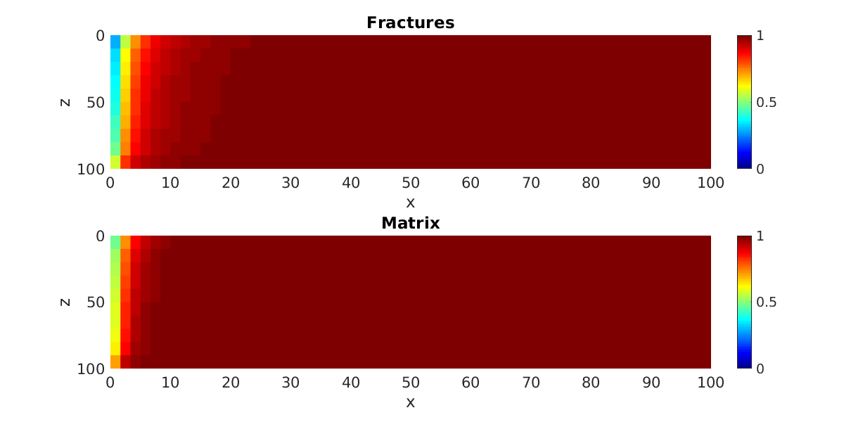
Two-phase gas injection in a water-saturated dual-porosity reservoir.¶

Generated from example_2ph_drainage.m

Gas flows in the fracture system, and transfer to the matrix happens via gravity drainage.

clear;
clc;
close all;

mrstModule add ad-blackoil ad-core ad-props dual-porosity

Set up grid¶

G = cartGrid([60, 1, 10], [100, 1, 100]*meter);
G = computeGeometry(G);

Set up rock properties¶

rock_matrix = makeRock(G, 10*milli*darcy, .1);
rock_fracture = makeRock(G, 100*milli*darcy, .01);

Set up fluid¶

fluid_matrix = initSimpleADIFluid('phases', 'WO', 'c', [1e-12;1e-12],...
                                  'rho',[1000,1]);
fluid_fracture = initSimpleADIFluid('phases', 'WO', 'c', [1e-12;1e-12],...
                                  'rho',[1000,1]);

Set the DP model. Here, a two-phase model is used. Rock and fluid¶

are sent in the constructor as a cell array {fracture,matrix}. We use and OilWater model, where oil plays the role of the gas.

gravity on;
model = TwoPhaseOilWaterModelDP(G, {rock_fracture,rock_matrix},...
                                      {fluid_fracture,fluid_matrix});

Setting transfer function. This step is important to ensure that fluids¶

will be transferred from fracture to matrix (and vice-versa). There are several options of shape factor (see folder transfer_models/shape_factor_models/) that could be set in this constructor. The second argument is the matrix block size.

model.transfer_model_object = EclipseTwoPhaseTransferFunction('CoatsShapeFactor',[1,1,10]);

Initializing state¶

state = initResSol(G, 0*psia, [1,0]);
state.wellSol = initWellSolAD([], model, state);
state.pressure_matrix = state.pressure;
state.sm = state.s;

Boundary conditions¶

bc = pside([], G, 'xmax', 0*psia, 'sat', [0,1]);
bc = pside(bc, G, 'xmin', 500*psia, 'sat', [0,1]);

Solver¶

solver = NonLinearSolver();

Validating model¶

model = model.validateModel();

Figure¶

fig1 = figure('Position',[100,100,1200,600]);
fig1.Color = 'w';
colormap('jet');

Time loop¶

dt = 5*day;
tmax = 100*dt;
t = 0;
while t<=tmax

    disp(['Time = ',num2str(t/day), ' days'])
    state = solver.solveTimestep(state, dt, model, 'bc', bc);

    figure(fig1)
    subplot(2,1,1);
    p = plotCellData(G,state.s(:,1));
    p.EdgeAlpha = 0;
    view(0,0);
    colorbar;
    caxis([0,1]);
    set(gca,'FontSize',16);
    xlabel('x')
    zlabel('z')
    title('Fractures');

    subplot(2,1,2);
    p = plotCellData(G,state.sm(:,1));
    p.EdgeAlpha = 0;
    view(0,0);
    colorbar;
    caxis([0,1]);
    set(gca,'FontSize',16);
    xlabel('x')
    zlabel('z')
    title('Matrix');

    drawnow;

    t = t+dt;

end

Time = 0 days
Time = 5 days
Time = 10 days
Time = 15 days
Time = 20 days
Time = 25 days
Time = 30 days
Time = 35 days
...

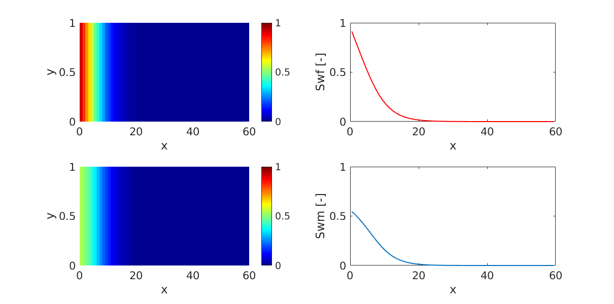
Two-phase water injection in an oil-saturated dual-porosity reservoir.¶

Generated from example_2ph_imbibition.m

Water flows quickly in the fracture system, while transfer to the matrix happens via spontaneous imbibition.

clear;
clc;
close all;

mrstModule add ad-blackoil ad-core ad-props dual-porosity

Set up grid¶

G = cartGrid([60, 1, 1], [60, 1, 1]*meter);
G = computeGeometry(G);

Set up rock properties¶

rock_matrix = makeRock(G, 10*milli*darcy, .1);
rock_fracture = makeRock(G, 100*milli*darcy, .01);

Set up fluid¶

fluid_matrix = initSimpleADIFluid('phases', 'WO', 'c', [1e-12;1e-12]);
fluid_fracture = initSimpleADIFluid('phases', 'WO', 'c', [1e-12;1e-12]);
Pe = 100*psia;
fluid_matrix.pcOW = @(sw)Pe;

Set the DP model. Here, a two-phase model is used. Rock and fluid¶

are sent in the constructor as a cell array {fracture,matrix}

model = TwoPhaseOilWaterModelDP(G, {rock_fracture,rock_matrix},...
                                   {fluid_fracture,fluid_matrix});

Setting transfer function. This step is important to ensure that fluids¶

will be transferred from fracture to matrix (and vice-versa). There are several options of shape factor (see folder transfer_models/shape_factor_models/) that could be set in this constructor. The second argument is the matrix block size. Another possible transfer function to be used in this model would be: model.transfer_model_object = EclipseTransferFunction();

model.transfer_model_object = KazemiTwoPhaseTransferFunction('KazemiShapeFactor',...
                                                              [5,5,5]);

Initializing state¶

state = initResSol(G, 0*psia, [0,1]);
state.wellSol = initWellSolAD([], model, state);
state.pressure_matrix = state.pressure;
state.sm = state.s;

Boundary conditions¶

bc = pside([], G, 'xmax', 0*psia, 'sat', [1,0]);
bc = pside(bc, G, 'xmin', 1000*psia, 'sat', [1,0]);

Solver¶

solver = NonLinearSolver();

Validating model¶

model = model.validateModel();

Figure¶

fig1 = figure('Position',[100,100,1200,600]);
fig1.Color = 'w';
colormap('jet');

Time loop¶

dt = 5*day;
tmax = 100*dt;
t = 0;
while t<=tmax

    disp(['Time = ',num2str(t/day), ' days'])
    state = solver.solveTimestep(state, dt, model, 'bc', bc);

    figure(fig1)
    subplot(2,2,1);
    p = plotCellData(G,state.s(:,1));
    p.EdgeAlpha = 0;
    colorbar;
    caxis([0,1]);
    set(gca,'FontSize',16);
    xlabel('x')
    ylabel('y')

    subplot(2,2,3);
    p = plotCellData(G,state.sm(:,1));
    p.EdgeAlpha = 0;
    colorbar;
    caxis([0,1]);
    set(gca,'FontSize',16);
    xlabel('x')
    ylabel('y')

    figure(fig1)
    subplot(2,2,2);
    plot(G.cells.centroids(:,1),state.s(:,1),'LineWidth',1.5,'Color','r');
    set(gca,'FontSize',16);
    xlabel('x')
    ylim([0,1])
    ylabel('Swf [-]')

    subplot(2,2,4);
    plot(G.cells.centroids(:,1),state.sm(:,1),'LineWidth',1.5);
    set(gca,'FontSize',16);
    xlabel('x')
    ylim([0,1])
    ylabel('Swm [-]')

    drawnow;

    t = t+dt;

end

Time = 0 days
Time = 5 days
Time = 10 days
Time = 15 days
Time = 20 days
Time = 25 days
Time = 30 days
Time = 35 days
...

dual-porosity: Dual porosity/permeability model for fractures¶

MRST’s Dual-Porosity Module¶

Examples¶

Single-phase depletion of a dual-porosity reservoir. Fracture fluid is¶

Set up grid¶

Set up rock properties¶

Set up fluid¶

Set the DP model. Here, a single-phase model is used. Rock and fluid¶

Setting transfer function. This step is important to ensure that fluids¶

Initializing state¶

Boundary conditions¶

Solver¶

Validating model¶

Figure¶

Time loop¶

Two-phase gas injection in a water-saturated dual-porosity reservoir.¶

Set up grid¶

Set up rock properties¶

Set up fluid¶

Set the DP model. Here, a two-phase model is used. Rock and fluid¶

Setting transfer function. This step is important to ensure that fluids¶

Initializing state¶

Boundary conditions¶

Solver¶

Validating model¶

Figure¶

Time loop¶

Two-phase water injection in an oil-saturated dual-porosity reservoir.¶

Set up grid¶

Set up rock properties¶

Set up fluid¶

Set the DP model. Here, a two-phase model is used. Rock and fluid¶

Setting transfer function. This step is important to ensure that fluids¶

Initializing state¶

Boundary conditions¶

Solver¶

Validating model¶

Figure¶

Time loop¶

`dual-porosity`: Dual porosity/permeability model for fractures¶