`ad-core`: Automatic Differentiation Core¶

Object-oriented framework for solvers based on automatic differentiation (MRST AD-OO). This module by itself does not contain any complete simulators, but rather implements the common framework used for many other modules. For instance, the ad-blackoil module contains models for black-oil equations that inherit all basic features from ad-core, the ad-eor module inherits models from ad-blackoil, and so on.

Overview of the solvers:

Models¶

Base classes¶

Contents¶

MODELS

Files: ExtendedReservoirModel - PhysicalModel - Base class for all AD models. Implements a generic discretized model. ReservoirModel - Base class for physical models WrapperModel - Wrapper model which can be inherited for operations on the parent

class PhysicalModel(G, varargin)¶

Base class for all AD models. Implements a generic discretized model.

Synopsis:

model = PhysicalModel(G)

Description:

Base class for implementing physical models for use with automatic differentiation. This class cannot be used directly.

A physical model consists of a set of discrete operators that can be used to define the model equations and a nonlinear tolerance that defines how close the values must be to zero before the equations can be considered to be fulfilled. In most cases, the operators are defined over a grid, which is an optional property in this class. In addition, the class contains a flag informing if the model equations are linear, and a flag determining verbosity of class functions.

The class contains member functions for:

evaluating residual equations and Jacobians

querying and setting individual variables in the physical state

executing a single nonlinear step (i.e., a linear solve with a possible subsequent stabilization step), verifying convergence, and reporting the status of the step

verifying the model, associated physical states, or individual physical properties

as well as a number of utility functions for updating the physical state with increments from the linear solve, etc. See the implementation of the class for more details.

Keyword Arguments:
Parameters:	G – Simulation grid. Can be set to empty.
	‘property’ – Set property to the specified value.
Returns:	model – Class instance of `PhysicalModel`.

Note

This is the standard base class for the AD-OO solvers. As such, it does not implement any specific discretization or equations and is seldom instansiated on its own.

See also

ReservoirModel, ThreePhaseBlackOilModel, TwoPhaseOilWaterModel

capProperty(model, state, name, minvalue, maxvalue)¶

Ensure that a property is within a specific range by capping.

Synopsis:

state = model.capProperty(state, 'someProp', minValOfProp)
state = model.capProperty(state, 'someProp', minValOfProp, maxValOfProp)

Parameters:

model – Class instance.
state – State `struct`to be updated.
name – Name of the field to update, as supported by model.getVariableField.
minvalue – Minimum value of state property name. Any values below this threshold will be set to this value. Set to -inf for no lower bound.
maxvalue – OPTIONAL: Maximum value of state property name. Values that are larger than this limit are set to the limit. For no upper limit, set inf.

Returns:

state – State struct where name is within the limits.

Example:

% Make a random field, and limit it to the range [0.2, 0.5].
state = struct('pressure', rand(10, 1))
state = model.capProperty(state, 0.2, 0.5);
disp(model.getProp(state, 'pressure'))

checkConvergence(model, problem, varargin)¶

Check and report convergence based on residual tolerances

Synopsis:

[convergence, values, names] = model.checkConvergence(problem)

Description:

Basic convergence testing for a linearized problem. By default, this simply takes the inf norm of all model equations. Subclasses are free to overload this function for more sophisticated and robust options.

Parameters:	model – Class instance problem – `LinearizedProblemAD` to be checked for convergence. The default behavior is to check all equations against `model.nonlinearTolerance` in the inf/max norm. n – OPTIONAL· The norm to be used. Default: `inf`.
Returns:	convergence – Vector of length `N` with bools indicating `true/false` if that residual/error measure has converged. values – Vector of length `N` containing the numerical values checked for convergence. names – Cell array of length `N` containing the names tested for convergence.

Note

By default, N is equal to the number of equations in problem and the convergence simply checks the convergence of each equation against a generic nonlinearTolerance. However, subclasses are free to produce any number of convergence criterions and they need not correspond to specific equations at all.

checkProperty(model, state, property, n_el, dim)¶

Check dimensions of property and throw error if dims do not match

Synopsis:

model.checkProperty(state, 'pressure', G.cells.num, 1);
model.checkProperty(state, 'components', [ncell, ncomp], [1, 2]);

Parameters:	model – Class instance. state – State `struct`to be checked. name – Name of the field to check, as supported by `model.getVariableField`. n_el – Array of length `N` where entry i`corresponds to the size of the property in dimension `dim(i). dim – Array of length `N` corresponding to the dimensions for which `n_el` is to be checked.

getAdjointEquations(model, state0, state, dt, forces, varargin)¶

Get the adjoint equations (please read note before use!)

Synopsis:

[problem, state] = model.getAdjointEquations(state0, state, dt, drivingForces)

Description:

Function to get equation when using adjoint to calculate gradients. This make it possible to use different equations to calculate the solution in the forward mode, for example if equations are solved explicitly as for hysteretic models. it is assumed that the solution of the system in forward for the two different equations are equal i.e problem.val == 0.

Keyword Arguments:
Parameters:	model – Class instance state – Current state to be solved for time t + dt. state0 – The converged state at time t. dt – The scalar time-step. forces – Forces struct. See `getDrivingForces`.
Returns:	problem – `LinearizedProblemAD` derived class containing the linearized equations used for the adjoint problem. This function is normally `getEquations` and assumes that the function supports the `reverseMode` argument. state – State. Possibly updated. See `getEquations` for details.
	‘reverseMode’ – If set to true, the reverse mode of the equations are provided.

Note

A caveat is that this function provides the forward-mode version of the adjoint equations, normally identical to getEquations. MRST allows for separate implementations of adjoint and regular equations in order to allow for rigorous treatment of hysteresis and other semi-explicit parameters.

getDrivingForces(model, control)¶

Get driving forces in expanded format.

Synopsis:

vararg = model.getDrivingForces(schedule.control(ix))

Parameters:

model – Class instance
control – Struct with the driving forces as fields. This should be a struct with the same fields as in getValidDrivingForces, although this is not explicitly enforced in this routine.

Returns:

vararg –

Cell-array of forces in the format:

{'W', W, 'bc', bc, ...}

This is typically used as input to variable input argument functions that support various boundary conditions options.

getEquations(model, state0, state, dt, forces, varargin)¶

Get the set of linearized model equations with possible Jacobians

Synopsis:

[problem, state] = model.getEquations(state0, state, dt, drivingForces)

Description:

Provide a set of linearized equations. Unless otherwise noted, these equations will have ADI type, containing both the value and Jacobians of the residual equations.

Keyword Arguments:
Parameters:	model – Class instance state – Current state to be solved for time t + dt. state0 – The converged state at time t. dt – The scalar time-step. forces – Forces struct. See `getDrivingForces`.
	‘resOnly’ – If supported by the equations, this flag will result in only the values of the equations being computed, omitting any Jacobians. ‘iteration’ – The nonlinear iteration number. This can be provided so that the underlying equations can account for the progress of the nonlinear solution process in a limited degree, for example by updating some quantities only at the first iteration.
Returns:	problem – Instance of the wrapper class `LinearizedProblemAD` containing the residual equations as well as other useful information. state – The equations are allowed to modify the system state, allowing a limited caching of expensive calculations only performed when necessary.

See also

getAdjointEquations

getIncrement(model, dx, problem, name)¶

Get specific named increment from a list of different increments.

Synopsis:

dv = model.getIncrement(dx, problem, 'name')

Description:

Find increment in linearized problem with given name, or output zero if not found. A linearized problem can give updates to multiple variables and this makes it easier to get those values without having to know the order they were input into the constructor.

Parameters:	model – Class instance. dx – Cell array of increments corresponding to the names in `problem.primaryVariables`. problem – Instance of `LinearizedProblem` from which the increments were computed. name – Name of the variable for which the increment is to be extracted.
Returns:	dv – The value of the increment, if it is found. Otherwise a scalar zero value is returned.

getMaximumTimestep(model, state, state0, dt, drivingForces)¶: Define the maximum allowable time-step based on physics or discretization choice

getModelEquations(model, state0, state, dt, drivingForces)¶: Get equations from AD states

getPrimaryVariables(model, state)¶: Get primary variables from state

getProp(model, state, name)¶

Get a single property from the nonlinear state

Synopsis:

p = model.getProp(state, 'pressure');

Parameters:	model – Class instance. state – `struct` holding the state of the nonlinear problem. name – A property name supported by the model’s `getVariableField` mapping.
Returns:	p – Property taken from the state. state – The state (modified if property evaluation was done)

See also

getProps

getProps(model, state, varargin)¶

Get multiple properties from state in one go

Synopsis:

[p, s] = model.getProps(state, 'pressure', 's');

Keyword Arguments:
Parameters:	model – Class instance. state – `struct` holding the state of the nonlinear problem.
	‘FieldName’ – Property names to be extracted. Any number of properties can be requested.
Returns:	varargout – Equal number of output arguments to the number of property strings sent in, corresponding to the respective properties.

See also

getProp

getValidDrivingForces(model)¶

Get a struct with the default valid driving forces for the model

Synopsis:

forces = model.getValidDrivingForces();

Description:

Different models support different types of boundary conditions. Each model should implement a default struct, showing the solvers what a typical allowed struct of boundary conditions looks like in terms of the named fields present.

Parameters:	model – Class instance
Returns:	forces – A struct with any number of fields. The fields must be present, but they can be empty.

getVariableField(model, name, throwError)¶

Map known variable by name to field and column index in state

Synopsis:

[fn, index] = model.getVariableField('someKnownField')

Description:

Get the index/name mapping for the model (such as where pressure or water saturation is located in state). For this parent class, this always result in an error, as this model knows of no variables.

For subclasses, however, this function is the primary method the class uses to map named values (such as the name of a component, or the human readable name of some property) and the compact representation in the state itself.

Parameters:	model – Class instance. name – The name of the property for which the storage field in `state` is requested. Attempts at retrieving a field the model does not know results in an error. throwError – OPTIONAL: If set to false, no error is thrown and empty fields are returned.
Returns:	fn – Field name in the `struct` where `name` is stored. index – Column index of the data.

See also

getProp, setProp

incrementProp(model, state, name, increment)¶

Increment named state property by given value

Synopsis:

state = model.incrementProp(state, 'PropertyName', increment)

Parameters:	model – Class instance. state – `struct` holding the state of the nonlinear problem. name – Name of the property to updated. See `getVariableField` value – The increment that will be added to the current value of property `name`.
Returns:	state – Updated state `struct`.

Example:

% For a model which knows of the field 'pressure', increment
% the value by 7 so that the final value is 10 (=3+7).
state = struct(‘pressure’, 3);
state = model.incrementProp(state, ‘pressure’, 7);

initStateAD(model, state, vars, names, origin)¶: Initialize AD state from double state

static limitUpdateAbsolute(dv, maxAbsCh)¶: Limit a update by absolute limit

static limitUpdateRelative(dv, val, maxRelCh)¶: Limit a update by relative limit

makeStepReport(model, varargin)¶

Get the standardized report all models provide from stepFunction

Synopsis:

report = model.makeStepReport('Converged', true);

Description:

Normalized struct with a number of useful fields. The most important fields are the fields representing Failure and Converged which NonLinearSolver reacts appropriately to.

Keyword Arguments:
Parameters:	model – Class instance
	various – Keyword/value pairs that override the default values.
Returns:	report – Normalized report with defaulted values where not provided.

See also

stepFunction, NonLinearSolverAD

prepareReportstep(model, state, state0, dT, drivingForces)¶: Prepare state and model (temporarily) before solving a report-step

prepareTimestep(model, state, state0, dt, drivingForces)¶

Prepare state and model (temporarily) before solving a time-step

Synopsis:

[model, state] = model.prepareTimestep(state, state0, dt, drivingForces)

Description:

Prepare model and state just before the first call to stepFunction in a solution loop.

Parameters:

model – Class instance
state – struct representing the current state of the solution variables to be updated.
problem – LinearizedProblemAD instance that has primaryVariables which matches dx in length and meaning.
dx – Cell-wise increments. These are typically output from LinearSolverAD.solveLinearizedProblem.
forces – The forces used to produce the update. See getDrivingForces.

Returns:

model – Updated model (non-persistent)
state – Updated state with physically reasonable values.

Note

Any changes to the model are temporary for this specific step, as enforced by the NonLinearSolver. Any changes will not apply to the next time-step.

reduceState(model, state, removeContainers)¶: Reduce state to doubles, and optionally remove the property containers to reduce storage space

setProp(model, state, name, value)¶

Set named state property to given value

Synopsis:

state = model.setProp(state, 'PropertyName', value)

Parameters:	model – Class instance. state – `struct` holding the state of the nonlinear problem. name – Name of the property to updated. See `getVariableField` value – The updated value that will be set.
Returns:	state – Updated state `struct`.

Example:

% This will set state.pressure to 5 if the model knows of a
% state field named pressure. If it is not known, it will
% result in an error.
state = struct('pressure', 0);
state = model.setProp(state, 'pressure', 5);

solveAdjoint(model, solver, getState, getObj, schedule, gradient, stepNo)¶

Solve a single linear adjoint step to obtain the gradient

Synopsis:

gradient = model.solveAdjoint(solver, getState, ...
                        getObjective, schedule, gradient, itNo)

Description:

This solves the linear adjoint equations. This is the backwards analogue of the forward mode stepFunction in PhysicalModel as well as the solveTimestep method in NonLinearSolver.

Parameters:

model – Class instance.
solver – Linear solver to be used to solve the linearized system.
getState –
Function handle. Should support the syntax:
```
state = getState(stepNo)
```
To obtain the converged state from the forward simulation for step stepNo.
getObj –
Function handle providing the objective function for a specific step stepNo:
```
objfn = getObj(stepNo)
```
schedule – Schedule used to compute the forward simulation.
gradient – Current gradient to be updated. See outputs.
stepNo – The current control step to be solved.

Returns:

gradient – The updated gradient.
result – Solution of the adjoint problem.
report – Report with information about the solution process.

See also

computeGradientAdjointAD

stepFunction(model, state, state0, dt, drivingForces, linsolver, nonlinsolver, iteration, varargin)¶

Perform a step that ideally brings the state closer to convergence

Synopsis:

[state, report] = model.stepFunction(state, state0, dt, ...
                                     forces, ls, nls, it)

Description:

Perform a single nonlinear step and report the progress towards convergence. The exact semantics of a nonlinear step varies from model to model, but the default behavior is to linearize the equations and solve a single step of the Newton-Rapshon algorithm for general nonlinear equations.

updateAfterConvergence(model, state0, state, dt, drivingForces)¶

Final update to the state after convergence has been achieved

Synopsis:

[state, report] = model.updateAfterConvergence(state0, state, dt, forces)

Description:

Update state based on nonlinear increment after timestep has converged. Defaults to doing nothing since not all models require this.

This function allows for the update of secondary variables instate after convergence has been achieved. This is especially useful for hysteretic parameters, where future function evaluations depend on the previous maximum value over all converged states.

Parameters:	model – Class instance. state – `struct` holding the current solution state. forces – Driving forces used to execute the step. See `getDrivingForces`.
Returns:	state – Updated `struct` holding the current solution state. report – Report containing information about the update.

updateForChangedControls(model, state, forces)¶

Update model and state when controls/drivingForces has changed

Synopsis:

[model, state] = model.updateForChangedControls(state, forces)

Description:

Whenever controls change, this function should ensure that both model and state are up to date with the present set of driving forces.

Parameters:	model – Class instance. state – `struct` holding the current solution state. forces – The new driving forces to be used in subsequent calls to `getEquations`. See `getDrivingForces`.
Returns:	model – Updated class instance. state – Updated `struct` holding the current solution state with accomodations made for any changed controls that provide e.g. primary variables.

updateState(model, state, problem, dx, forces)¶

Update the state based on increments of the primary values

Synopsis:

[state, report] = model.updateState(state, problem, dx, drivingForces)

Description:

Update the state’s primary variables (and any secondary quantities computing during the update process) based on a set of increments to each of the primary variables contained in problem.primaryVariables.

This function should ensure that values are within physically meaningful values and are meaningful so that the next call to stepFunction can produce yet another set of reasonable increments in a process that eventually results in convergence.

Parameters:

model – Class instance
state – struct representing the current state of the solution variables to be updated.
problem – LinearizedProblemAD instance that has primaryVariables which matches dx in length and meaning.
dx – Cell-wise increments. These are typically output from LinearSolverAD.solveLinearizedProblem.
forces – The forces used to produce the update. See getDrivingForces.

Returns:

state – Updated state with physically reasonable values.
report – Struct with information about the update process.

Note

Specific properties can be manually updated with a variety of different functions. We trust the user and leave these functions as public. However, the main gateway to the update of state is through this function to ensure that all values are updated simultaneously. For many problems, updates can not be done separately and all changes in the primary variables must considered together for the optimal performance.

updateStateFromIncrement(model, state, dx, problem, name, relchangemax, abschangemax)¶

Update value in state, with optional limits on update magnitude

Synopsis:

state = model.updateStateFromIncrement(state, dx, problem, 'name')
[state, val, val0] = model.updateStateFromIncrement(state, dx, problem, 'name', 1, 0.1)

Parameters:

model – Class instance.
state – State `struct`to be updated.
dx – Increments. Either a cell array matching the the primary variables of problem, or a single value.
problem – LinearizedProblem used to obtain the increments. This input argument is only used if dx is a cell array and can be replaced by a dummy value if dx is a numerical type.
name – Name of the field to update, as supported by model.getVariableField.
relchangemax – OPTIONAL. If provided, this will be interpreted as the maximum relative change in the variable allowed.
abschangemax – OPTIONAL. If provided, this is the maximum absolute change in the variable allowed.

Returns:

state – State with updated value.

Example:

% Update pressure with an increment of 10, without any limits,
% resulting in the pressure being 110 after the update.
state = struct('pressure', 10);
state = model.updateStateFromIncrement(state, 100, problem, 'pressure')
% Alternatively, we can use a relative limit on the update. In
% the following, the pressure will be set to 11 as an immediate
% update to 110 would violate the maximum relative change of
% 0.1 (10 %)
 state = model.updateStateFromIncrement(state, 100, problem, 'pressure', .1)

Note

Relative limits such as these are important when working with tabulated and nonsmooth properties in a Newton-type loop, as the initial updates may be far outside the reasonable region of linearization for a complex problem. On the other hand, limiting the relative updates can delay convergence for smooth problems with analytic properties and will, in particular, prevent zero states from being updated, so use with care.

validateModel(model, varargin)¶

Validate model and check if it is ready for simulation

Synopsis:

model = model.validateModel();
model = model.validateModel(forces);

Description:

Validate that a model is suitable for simulation. If the missing or inconsistent parameters can be fixed automatically, an updated model will be returned. Otherwise, an error should occur.

Second input may be the forces struct argument. This function should NOT require forces arg to run, however.

Parameters:	model – Class instance to be validated. forces – (OPTIONAL): The forces to be used. Some models require setup and configuration specific to the forces used. This is especially important for the `FacilityModel`, which implements the coupling between wells and the reservoir for `ReservoirModel` subclasses of `PhysicalModel`.
Returns:	model – Class instance. If returned, this model is ready for simulation. It may have been changed in the process.

validateState(model, state)¶

Validate state and check if it is ready for simulation

Synopsis:

state = model.validateState(state);

Description:

Validate the state for use with model. Should check that required fields are present and of the right dimensions. If missing fields can be assigned default values, state is return with the required fields added. If reasonable default values cannot be assigned, a descriptive error should be thrown telling the user what is missing or wrong (and ideally how to fix it).

Parameters:	model – Class instance for which `state` is intended as a valid state. state – `struct` which is to be validated.
Returns:	state – `struct`. If returned, this state is ready for simulation with `model`. It may have been changed in the process.

G = None¶: Grid. Can be empty.

nonlinearTolerance = None¶: Inf norm tolerance for checking residuals

operators = None¶: Operators used for construction of systems

stepFunctionIsLinear = None¶: Model step function is linear.

verbose = None¶: Verbosity from model routines

class ReservoirModel(G, varargin)¶

Bases: PhysicalModel

Base class for physical models

Synopsis:

model = ReservoirModel(G, rock, fluid)

Description:

Extension of PhysicalModel class to accomodate reservoir-specific features such as fluid and rock as well as commonly used phases and variables.

Keyword Arguments:
Parameters:	G – Simulation grid. rock – Valid rock used for the model. fluid – Fluid model used for the model.
	‘property’ – Set property to the specified value.
Returns:	Class instance.

See also

ThreePhaseBlackOilModel, TwoPhaseOilWaterModel, PhysicalModel

addBoundaryConditionsAndSources(model, eqs, names, types, state, p, s, mob, rho, dissolved, components, forces)¶

Add in the boundary conditions and source terms to equations

Synopsis:

[eqs, state] = addBoundaryConditionsAndSources(model, eqs, names, types, state, ...
                                                     p, sat, mob, rho, ...
                                                     rs, components, ...
                                                     drivingForces);

Parameters:

model – Class instance.
eqs – Cell array of equations that are to be updated.
names – The names of the equations to be updated. If phase-pseudocomponents are to be used, the names must correspond to some combination of “water”, “oil”, “gas” if no special component treatment is to be introduced.
types – Cell array with the types of “eqs”. Note that these types must be ‘cell’ where source terms is to be added.
src – Struct containing all the different source terms that were computed and added to the equations.
p – Cell array of phase pressures.
s – Cell array of phase saturations.
mob – Cell array of phase mobilities
rho – Cell array of phase densities
dissolved – Cell array of dissolved components for black-oil style pseudocompositional models.
components – Cell array of equal length to the number of components. The exact representation may vary based on the model, but the respective sub-component is passed onto addComponentContributions.
forces – DrivingForces struct (see getValidDrivingForces) containing (possibily empty) src and bc fields.

Returns:

eqs – Equations with corresponding source terms added.
state – Reservoir state. Can be modified to store e.g. boundary fluxes due to boundary conditions.
src – Normalized struct containing the source terms used.

Note

This function accomodates both the option of black-oil pseudocomponents (if the model equations are named “oil”, “gas” or water) and true components existing in multiple phases. Mixing the two behaviors can lead to unexpected source terms.

addComponentContributions(model, cname, eq, component, src, force)¶

For a given component conservation equation, compute and add in source terms for a specific source/bc where the fluxes have already been computed.

Parameters:

model – (Base class, automatic)
cname – Name of the component. Must be a property known to the model itself through getProp and getVariableField.
eq – Equation where the source terms are to be added. Should be one value per cell in the simulation grid (model.G) so that the src.sourceCells is meaningful.
component – Cell-wise values of the component in question. Used for outflow source terms only.
src – Source struct containing fields for fluxes etc. Should be constructed from force and the current reservoir state by computeSourcesAndBoundaryConditionsAD.
force – Force struct used to produce src. Should contain the field defining the component in question, so that the inflow of the component through the boundary condition or source terms can accurately by estimated.

static adjustStepFromSatBounds(s, ds)¶: Ensure that cellwise increment for each phase is done with the same length, in a manner that avoids saturation violations.

compVarIndex(model, name)¶

Find the index of a component variable by name

Synopsis:

index = model.compVarIndex('co2')

Parameters:	model – Class instance name – Name of component.
Returns:	index – Index of the component for this model. Empty if saturation was not known to model.

evaluateRelPerm(model, sat, varargin)¶

Evaluate relative permeability corresponding to active phases

Synopsis:

% Single-phase water model
krW = model.evaluateRelPerm({sW});
% Two-phase oil-water model
[krW, krO] = model.evaluateRelPerm({sW, sO});
% Two-phase water-gas model
[krW, krG] = model.evaluateRelPerm({sW, sG});
% Three-phase oil-water-gas model
[krW, krO, krG] = model.evaluateRelPerm({sW, sO, sG});

Parameters:	model – The model sat – Cell array containing the saturations for all active phases.
Returns:	varargout – One output argument per phase present, corresponding to evaluated relative permeability functions for each phase in the canonical ordering.

See also

relPermWOG, relPermWO, relPermOG, relPermWG

getActivePhases(model)¶

Get active flag for MRST’s canonical phase ordering (WOG)

Synopsis:

[act, indices] = model.getActivePhases();

Parameters:	model – Class instance
Returns:	isActive – Total number of known phases array with booleans indicating if that phase is present. MRST uses a ordering of water, oil and then gas. phInd – Indices of the phases present. For instance, if water and gas are the only ones present, `phInd = [1, 3]`

getComponentNames(model)¶

#ok Get the names of components for the model .. rubric:: Synopsis:

names = model.getComponentNames();

Parameters:	model – Class instance.
Returns:	names – Cell array of component names in no particular order.

getConvergenceValues(model, problem, varargin)¶: Check convergence criterion. Relies on FacilityModel to check wells.

See also

ad_core.models.PhysicalModel.checkConvergence

getExtraWellContributions(model, well, wellSol0, wellSol, q_s, bh, packed, qMass, qVol, dt, iteration)¶

This function is called by the well model (base class: SimpleWell) during the assembly of well equations and addition of well source terms. The purpose of this function, given the internal variables of the well model, is to compute the additional closure equations and source terms that the model requires. For instance, if the model contains different components that require special treatment (see for example the implementation of this function in ad_eor.models.OilWaterPolymerModel in the ad-eor module), this function should assemble any additional equations and corresponding source terms. It is also possible to add source terms without actually adding well equations.

Returns:

compEqs – A cell array of additional equations added to the system to account for the treatment of components etc in the well system.
compSrc – Cell array of component source terms, ordered and with the same length as the output from ReservoirModel.getComponentNames.
eqNames – Names of the added equations. Must correspond to the same entries as getExtraWellEquationNames (but does not have to maintain the same ordering).

Note

Input arguments are intentionally undocumented and subject to change. Please see SimpleWell for details.

getExtraWellEquationNames(model)¶

Get the names and types of extra well equations in model

Synopsis:

[names, types] = model.getExtraWellEquationNames();

Parameters:	model – Base class.
Returns:	names – Cell array of additional well equations. types – Cell array of corresponding types to `names`.

See also

getExtraWellContributions

getExtraWellPrimaryVariableNames(model)¶

Get the names of extra well primary variables required by model.

Synopsis:

names = model.getExtraWellPrimaryVariableNames();

Parameters:	model – Class instance
Returns:	names – Cell array of named primary variables.

See also

getExtraWellContributions

getGravityGradient(model)¶

Get the discretized gravity contribution on faces

Synopsis:

gdz = model.getGravityGradient();

Parameters:	model – Class instance
Returns:	g – One entry of the gravity contribution per face in the grid. Does not necessarily assume that gravity is aligned with one specific direction.

See also

gravity

getGravityVector(model)¶

Get the gravity vector used to instantiate the model

Synopsis:

g = model.getGravityVector();

Parameters:	model – Class instance
Returns:	g – `model.G.griddim` long vector representing the gravity accleration constant along increasing depth.

See also

gravity

getMaximumTimestep(model, state, state0, dt0, drivingForces)¶: Define the maximum allowable time-step based on physics or discretization choice

getPhaseIndex(model, phasename)¶

Query the index of a phase in the model’s ordering

Synopsis:

index = model.getPhaseNames();

Parameters:	model – Class instance phasename – The name of the phase to be found.
Returns:	index – Index of phase `phasename`

getPhaseIndices(model)¶: Get the active phases in canonical ordering

getPhaseNames(model)¶

Get short and long names of the present phases.

Synopsis:

[phNames, longNames] = model.getPhaseNames();

Parameters:	model – Class instance
Returns:	phNames – Cell array containing the short hanes (‘W’, ‘O’, G’) of the phases present longNames – Longer names (‘water’, ‘oil’, ‘gas’) of the phases present.

getScalingFactorsCPR(model, problem, names, solver)¶

#ok Get scaling factors for CPR reduction in CPRSolverAD

Parameters:	model – Class instance problem – `LinearizedProblemAD` which is intended for CPR preconditioning. names – The names of the equations for which the factors are to be obtained. solver – The `LinearSolverAD` class requesting the scaling factors.
Returns:	scaling – Cell array with either a scalar scaling factor for each equation, or a vector of equal length to that equation.

SEE ALSO: CPRSolverAD

getSurfaceDensities(model)¶

Get the surface densities of the active phases in canonical ordering (WOG, with any inactive phases removed).

Returns:	rhoS – pvt x n double array of surface densities.

getValidDrivingForces(model)¶: Get valid forces. This class adds support for wells, bc and src.

See also

ad_core.models.PhysicalModel.getValidDrivingForces

getVariableField(model, name, varargin)¶: Map variables to state field.

See also

ad_core.models.PhysicalModel.getVariableField

insertWellEquations(model, eqs, names, types, wellSol0, wellSol, wellVars, wellMap, p, mob, rho, dissolved, components, dt, opt)¶

Add in the effect of wells to a system of equations, by adding corresponding source terms and augmenting the system with additional equations for the wells.

Parameters:

eqs – Cell array of equations that are to be updated.
names – The names of the equations to be updated. If phase-pseudocomponents are to be used, the names must correspond to some combination of “water”, “oil”, “gas” if no special component treatment is to be introduced.
types – Cell array with the types of “eqs”. Note that these types must be ‘cell’ where source terms is to be added.
src – Struct containing all the different source terms that were computed and added to the equations.
various – Additional input arguments correspond to standard reservoir-well coupling found in `FacilityModel.

static relPermOG(so, sg, f, varargin)¶

Two-phase oil-gas relative permeability function

Synopsis:

[krO, krG] = model.relPermOG(so, sg, f);

Parameters:	sw – Water saturation sg – Gas saturation f – Struct representing the field. Fields that are used: `krO`: Oil relperm function of oil saturation. `krOG`: Oil-gas relperm function of gas saturation. This function is only used if `krO` is not found. `krG`: Gas relperm function of gas saturation.
Returns:	krO – Oil relative permeability. krG – Gas relative permeability

Note

This function should typically not be called directly as its interface is subject to change. Instead, use evaluateRelPerm.

static relPermWG(sw, sg, f, varargin)¶

Two-phase water-gas relative permeability function

Synopsis:

[krW, krG] = model.relPermWG(sw, sg, f);

Parameters:	sw – Water saturation sg – Gas saturation f – Struct representing the field. Fields that are used: `krW`: Water relperm function of water saturation. `krG`: Gas relperm function of gas saturation.
Returns:	krW – Water relative permeability. krG – Gas relative permeability

Note

This function should typically not be called directly as its interface is subject to change. Instead, use evaluateRelPerm.

static relPermWO(sw, so, f, varargin)¶

Two-phase water-oil relative permeability function

Synopsis:

[krW, krO] = model.relPermWO(sw, so, f);

Parameters:	sw – Water saturation so – Oil saturation f – Struct representing the field. Fields that are used: `krW`: Water relperm function of water saturation. `krO`: Oil relperm function of oil saturation. `krOW`: Oil-water relperm function of oil saturation. Only used if `krO` is not found.
Returns:	krW – Water relative permeability. krO – Oil relative permeability.

Note

This function should typically not be called directly as its interface is subject to change. Instead, use evaluateRelPerm.

static relPermWOG(sw, so, sg, f, varargin)¶

Three-phase water-oil-gas relative permeability function

Synopsis:

[krW, krO, krG] = model.relPermWOG(sw, so, sg, f);

Parameters:	sw – Water saturation so – Oil saturation sg – Gas saturation f – Struct representing the field. Fields that are used: `krW`: Water relperm function of water saturation. `krOW`: Oil-water relperm function of oil saturation. `krOG`: Oil-gas relperm function of oil saturation. `krG`: Gas relperm function of gas saturation. `sWcon`: Connate water saturation. OPTIONAL.
Returns:	krW – Water relative permeability. krO – Oil relative permeability. krG – Gas relative permeability

Note

This function should typically not be called directly as its interface is subject to change. Instead, use evaluateRelPerm.

satVarIndex(model, name)¶

Find the index of a saturation variable by name

Synopsis:

index = model.satVarIndex('water')

Parameters:	model – Class instance name – Name of phase.
Returns:	index – Index of the phase for this model. Empty if saturation was not found.

setPhaseData(model, state, data, fld, subs)¶

Store phase data in state for further output.

Synopsis:

state = model.setPhaseData(state, data, 'someField')
state = model.setPhaseData(state, data, 'someField', indices)

Description:

Utility function for storing phase data in the state. This is used for densities, fluxes, mobilities and so on when requested from the simulator.

Parameters:	model – Class instance data – Cell array of data to be stored. One entry per active phase in `model`. fld – The field to be stored. subs – OPTIONAL. The subset for which phase data is to be stored. Must be a valid index of the type data.(fld)(subs, someIndex) = data{i} for all i. Defaults to all indices.
Returns:	state – state with updated `fld`.

setupOperators(model, G, rock, varargin)¶

Set up default discretization operators and other static props

Synopsis:

model = model.setupOperators(G, rock)

Description:

This function calls the default set of discrete operators as implemented by setupOperatorsTPFA. The default operators use standard choices for reservoir simulation similar to what is found in commercial simulators: Single-point potential upwind and two-point flux approximation.

Parameters:	model – Class instance. G – The grid used for computing the operators. Must have geometry information added (typically from `computeGeometry`). Although this is a property on the model, we allow for passing of a different grid for the operator setup since this is useful in some workflows. rock – Rock structure. See `makeRock`.
Returns:	model – Model with updated `operators` property.

Note

This function is called automatically during class construction.

splitPrimaryVariables(model, vars)¶

Split cell array of primary variables into grouping .. rubric:: Synopsis:

[restVars, satVars, wellVars] = model.splitPrimaryVariables(vars)

Description:

Split a set of primary variables into three groups: Well variables, saturation variables and the rest. This is useful because the saturation variables usually are updated together, and the well variables are a special case.

Parameters:	model – Class instance. vars – Cell array with names of primary variables
Returns:	restVars – Names of variables that are not saturations or belong to the wells. satVars – Names of the saturation variables present in `vars`. wellVars – Names of the well variables present in `vars`

storeBoundaryFluxes(model, state, qW, qO, qG, forces)¶

Store integrated phase fluxes on boundary in state.

Synopsis:

Three-phase case
state = model.storeBoundaryFluxes(state, vW, vO, vG, forces);
% Only water and gas in model:
state = model.storeBoundaryFluxes(state, vW, [], vG, forces);

Parameters:	model – Class instance vW – Water fluxes, one value per BC interface. vO – Oil fluxes, one value per BC interface. vG – Gas fluxes, one value per BC interface. forces – `drivingForces` struct containing any boundary conditions used to obtain fluxes.
Returns:	state – State with stored values

See also

storeFluxes

storeDensity(model, state, rhoW, rhoO, rhoG)¶

Store phase densities per-cell in state.

Synopsis:

Three-phase case
state = model.storeDensity(state, rhoW, rhoO, rhoG);
% Only water and gas in model:
state = model.storeDensity(state, rhoW, [], rhoG);

Parameters:	model – Class instance rhoW – Water densities, one value per internal interface. rhoO – Oil densities, one value per internal interface. rhoG – Gas densities, one value per internal interface.
Returns:	state – State with stored values

See also

storeMobilities

storeFluxes(model, state, vW, vO, vG)¶

Store integrated internal phase fluxes in state.

Synopsis:

Three-phase case
state = model.storeFluxes(state, vW, vO, vG);
% Only water and gas in model:
state = model.storeFluxes(state, vW, [], vG);

Parameters:	model – Class instance vW – Water fluxes, one value per internal interface. vO – Oil fluxes, one value per internal interface. vG – Gas fluxes, one value per internal interface.
Returns:	state – State with stored values

See also

storeBoundaryFluxes

storeMobilities(model, state, mobW, mobO, mobG)¶

Store phase mobility per-cell in state.

Synopsis:

Three-phase case
state = model.storebfactors(state, mobW, mobO, mobG);
% Only water and gas in model:
state = model.storebfactors(state, mobW, [], mobG);

Parameters:	model – Class instance mobW – Water mobilities, one value per internal interface. mobO – Oil mobilities, one value per internal interface. mobG – Gas mobilities, one value per internal interface.
Returns:	state – State with stored values

See also

storeMobilities

storeUpstreamIndices(model, state, upcw, upco, upcg)¶

Store upstream indices for each phase in state.

Synopsis:

Three-phase case
state = model.storeUpstreamIndices(state, upcw, upco, upcg);
% Only water and gas in model:
state = model.storeUpstreamIndices(state, upcw, [], upcg);

Parameters:	model – Class instance upcw – Water upwind indicator, one value per internal interface. upco – Oil upwind indicator, one value per internal interface. upcg – Gas upwind indicator, one value per internal interface.
Returns:	state – State with stored values

See also

storeBoundaryFluxes, storeFluxes

storebfactors(model, state, bW, bO, bG)¶

Store phase reciprocal FVF per-cell in state.

Synopsis:

Three-phase case
state = model.storebfactors(state, bW, bO, bG);
% Only water and gas in model:
state = model.storebfactors(state, bW, [], bG);

Parameters:	model – Class instance bW – Water reciprocal FVF, one value per internal interface. bO – Oil reciprocal FVF, one value per internal interface. bG – Gas reciprocal FVF, one value per internal interface.
Returns:	state – State with stored values

See also

storeDensities

updateAfterConvergence(model, state0, state, dt, drivingForces)¶: Generic update function for reservoir models containing wells.

See also

ad_core.models.PhysicalModel.updateAfterConvergence

updateForChangedControls(model, state, forces)¶: Called whenever controls change.

Note

The addition this class makes is also updating the well solution and the underlying FacilityModel class instance.

See also

ad_core.models.PhysicalModel.updateForChangedControls

updateSaturations(model, state, dx, problem, satVars)¶

Update of phase-saturations

Synopsis:

state = model.updateSaturations(state, dx, problem, satVars)

Description:

Update saturations (likely state.s) under the constraint that the sum of volume fractions is always equal to 1. This assumes that we have solved for n - 1 phases when n phases are present.

Parameters:	model – Class instance state – State to be updated dx – Cell array of increments, some of which correspond to saturations problem – `LinearizedProblemAD` class instance from which `dx` was obtained. satVars – Cell array with the names of the saturation variables.
Returns:	state – Updated state with saturations within physical constraints.

See also

splitPrimaryVariables

updateState(model, state, problem, dx, drivingForces)¶: Generic update function for reservoir models containing wells.

See also

ad_core.models.PhysicalModel.updateState

validateModel(model, varargin)¶: Validate model.

See also

ad_core.models.PhysicalModel.validateModel

validateState(model, state)¶: Validate initial state.

See also

ad_core.models.PhysicalModel.validateState

FacilityModel = None¶: Facility model used to represent wells

FlowPropertyFunctions = None¶: Grouping for flow properties

FluxDiscretization = None¶: Grouping for flux discretization

dpMaxAbs = None¶: Maximum absolute pressure change

dpMaxRel = None¶: Maximum relative pressure change

dsMaxAbs = None¶: Maximum absolute saturation change

extraStateOutput = None¶: Write extra data to states. Depends on submodel type.

extraWellSolOutput = None¶: Output extra data to wellSols: GOR, WOR, …

fluid = None¶: The fluid model. See initSimpleADIFluid, initDeckADIFluid

gas = None¶: Indicator showing if the vapor/gas phase is present

gravity = None¶: Vector for the gravitational force

inputdata = None¶: Input data used to instantiate the model

maximumPressure = None¶: Maximum pressure allowed in reservoir

minimumPressure = None¶: Minimum pressure allowed in reservoir

oil = None¶: Indicator showing if the liquid/oil phase is present

outputFluxes = None¶: Store integrated fluxes in state.

rock = None¶: The rock structure (perm/poro/ntg). See makeRock.

useCNVConvergence = None¶: Use volume-scaled tolerance scheme

water = None¶: Indicator showing if the aqueous/water phase is present

class WrapperModel(parentModel, varargin)¶

Bases: PhysicalModel

Wrapper model which can be inherited for operations on the parent model.

prepareReportstep(model, state, state0, dt, drivingForces)¶: Prepare state and model (temporarily) before solving a report-step

prepareTimestep(model, state, state0, dt, drivingForces)¶: Prepare state and model (temporarily) before solving a time-step

Facility and wells¶

Contents¶

FACILITIES

Files: combineMSwithRegularWells - Combine regular and MS wells, accounting for missing fields computeWellContributionsSingleWell - Main internal function for computing well equations and source terms ExtendedFacilityModel - FacilityModel - A model coupling facilities and wells to the reservoir MultisegmentWell - Derived class implementing multisegment wells nozzleValve - Nozzle valve model packPerforationProperties - Extract variables corresponding to a specific well selectFacilityFromDeck - Pick FacilityModel from input deck setupMSWellEquationSingleWell - Setup well residual equations for multi-segmented wells - and only those. setupWellControlEquationsSingleWell - Setup well controll (residual) equations SimpleWell - Base class implementing a single, instantaneous equilibrium well model unpackPerforationProperties - Unpack the properties extracted by packPerforationProperties. Internal function. wellBoreFriction - Empricial model for well-bore friction UniformFacilityModel - Simplified facility model which is sometimes faster reorderWellPerforationsByDepth - Undocumented Utility Function

class FacilityModel(reservoirModel, varargin)¶

Bases: PhysicalModel

A model coupling facilities and wells to the reservoir

Synopsis:

model = FacilityModel(reservoirModel)

Description:

The FacilityModel is the layer between a ReservoirModel and the facilities. The facilities consist of a number of different wells that are implemented in their own subclasses.

Different wells have different governing equations, primary variables and convergence criterions. This class seamlessly handles wells appearing and disappearing, controls changing and even well type changing.

Keyword Arguments:
Parameters:	resModel – `ReservoirModel` derived class the facilities are coupled to.
	‘property’ – Set property to the specified value.
Returns:	model – Class instance of `FacilityModel`.

See also

ReservoirModel, PhysicalModel, SimpleWell

checkFacilityConvergence(model, problem)¶

Check if facility and submodels has converged

Synopsis:

[convergence, values, names, evaluated] = model. checkFacilityConvergence(problem)

Parameters:	model – Class instance. problem – `LinearizedProblemAD` to be checked for convergence.
Returns:	conv – Array of convergence flags for all tests. vals – Values checked to obtain `conv`. names – The names of the convergence checks/equations. eval – Logical array into problem.equations indicating which residual equations we have actually checked convergence for.

getActiveWellCells(model, wellSol)¶

Get the perforated cells in active wells

Synopsis:

wc = model.getActiveWellCells()

Parameters:	model – Facility model class instance.
Returns:	wc – Array of well cells that are active, and belong to active wells.

getAllPrimaryVariables(model, wellSol)¶

Get all primary variables (basic + extra)

Synopsis:

[variables, names, wellmap] = model.getAllPrimaryVariables(wellSol)

Description:

Gets all primary variables, both basic (rates, bhp) and added variables (added by different wells and from the model itself).

Parameters:

model – FacilityModel class instance
wellSol – The wellSol struct

Returns:

names – Cell array. Each cell is a string with the name of an variable.
variables – Column of cells. Each element, variables{i}, is a vector given the value corresponding to variable with name names{i}. This vector is composed of stacked values over all the wells that contains this variable.
wellmap – A combined struct containing mappings for both the standard and extra primary variables.

See also

getBasicPrimaryVariables, getExtraPrimaryVariables

getBasicPrimaryVariableNames(model)¶

Get the names of the basic primary variables present in all wells

Synopsis:

names = model.getBasicPrimaryVariableNames();

Description:

Get a list of the basic names of primary variables that will be required to solve a problem with the current set of wells. The basic primary variables are always present in MRST, and correspond to the phase rates for each phase present, as well as the bottom-hole pressures. This ensures that all solvers have a minimum feature set for well controls.

Parameters:	model – `FacilityModel` class instance
Returns:	names – Cell array of the names of the basic primary variables.

getBasicPrimaryVariables(model, wellSol)¶

Get the basic primary variables common to all well models.

Synopsis:

[vars, names, map] = model.getBasicPrimaryVariables(wellSol)

Description:

Get phase rates for the active phases and the bhp. In addition, the map contains indicators used to find the phase rates and BHP values in “variables” since these are of special importance to many applications and are considered canonical (i.e. they are always solution variables in MRST, and functions can assume that they will always be found in the variable set for wells).

Parameters:	model – `FacilityModel` class instance
Returns:	variables – Cell array of the primary variables. names – Cell array with the names of the primary variables. map – Struct with details on which variables correspond to ordered phase rates and the bottom hole pressures.

getEquations(model, state0, state, dt, drivingForces, varargin)¶

Get stand-alone equations for the wells

Synopsis:

[problem, state] = model.getEquations(state0, state, dt, drivingForces, varargin)

Description:

The well equations can be solved as a separate nonlinear system with the reservoir as a fixed quantity. This is useful for debugging.

Keyword Arguments:
Parameters:	model – `FacilityModel` instance. wellSol0 – wellSol struct at previous time-step. wellSol – wellSol struct at current time-step. dt – Time-step. forces – Forces struct for the wells.
	‘resOnly’ – If supported by the equations, this flag will result in only the values of the equations being computed, omitting any Jacobians. ‘iteration’ – The nonlinear iteration number. This can be provided so that the underlying equations can account for the progress of the nonlinear solution process in a limited degree, for example by updating some quantities only at the first iteration.
Returns:	problem – Instance of the wrapper class `LinearizedProblemAD` containing the residual equations as well as other useful information. state – The equations are allowed to modify the system state, allowing a limited caching of expensive calculations only performed when necessary.

getExtraPrimaryVariables(model, wellSol)¶

Get additional primary variables (not in the basic set)

Synopsis:

[variables, names, wellmap] = model.getExtraPrimaryVariables(wellSol)

Description:

Get extra primary variables are variables required by more advanced wells that are in addition to the basic facility variables (rates + bhp).

Parameters:

model – FacilityModel class instance
wellSol – The wellSol struct

Returns:

names – Column of cells. Each cell is a string with the name of an extra-variable.
variables – Column of cells. Each element, variables{i}, is a vector given the value corresponding to extra-variable with name names{i}. This vector is composed of stacked values over all the wells that contains this extra-variable.
wellmap – The facility model contains the extra-variables of all the well models that are used. Let us consider the well with well number wno (in the set of active wells), then the Well model is belongs to has its own extra-variables (a subset of those of the Facility model). We consider the j-th extra-variable of the Well model. Then, i = extraMap(wno, j) says that this extra-variable corresponds to names{i}.

See also

getBasicPrimaryVariables

getIndicesOfActiveWells(model, wellSol)¶

Get indices of active wells

Synopsis:

actIx = model.getIndicesOfActiveWells(wellSol);

Parameters:	model – `FacilityModel` class instance wellSol – The wellSol struct
Returns:	actIx – The indices of the active wells in the global list of all wells (active & inactive)

getNumberOfActiveWells(model, wellSol)¶

Get number of wells active initialized in facility

Synopsis:

W = model.getNumberOfActiveWells();

Parameters:	model – `FacilityModel` class instance
Returns:	nwell – Number of active wells

getNumberOfWells(model)¶

Get number of wells initialized in facility

Synopsis:

W = model.getNumberOfWells();

Parameters:	model – `FacilityModel` class instance
Returns:	nwell – Number of wells

getPrimaryVariableNames(model)¶

Get the names of primary variables present in all wells

Synopsis:

names = model.getPrimaryVariableNames();

Description:

Get a list of the names of primary variables that will be required to solve a problem with the current set of wells.

Parameters:	model – `FacilityModel` class instance
Returns:	names – Cell array of the names of the primary variables.

getValidDrivingForces(model)¶: Get valid driving forces.

See also

ad_core.models.PhysicalModel.getValidDrivingForces

getWellCells(model, subs)¶

Get the perforated cells of all wells, regardless of status

Synopsis:

wc = model.getWellCells()

Parameters:	model – Facility model class instance.
Returns:	wc – Array of well cells

getWellContributions(model, wellSol0, wellSol, wellvars, wellMap, p, mob, rho, dissolved, comp, dt, iteration)¶

Get sources, well equations and updated wellSol

Synopsis:

[sources, wellSystem, wellSol] = fm.getWellContributions(...
wellSol0, wellSol, wellvars, wellMap, p, mob, rho, dissolved, comp, dt, iteration)

Description:

Get the source terms due to the wells, control and well equations and updated well sol. Main gateway for adding wells to a set of equations.

Parameters:

model – Facility model class instance.
wellSol0 – wellSol struct at previous time-step.
wellSol – wellSol struct at current time-step.
wellvars – Well variables. Output from getAllPrimaryVariables.
wellMap – Well mapping. Output from getAllPrimaryVariables.
p – Pressure defined in all cells of the underlying ReservoirModel. Normally, this is the oil pressure.
mob – Cell array of phase mobilities defined in all cells of the reservoir.
rho – Cell array of phase densities defined in all cells of the reservoir.
dissolved – Black-oil style dissolution. See ad_blackoil.models.ThreePhaseBlackoilModel.getDissolutionMatrix.
comp – Cell array of components in the reservoir.
dt – The time-step.
iteration – The current nonlinear iteration for which the sources are to be computed.

Returns:

sources – Struct containing source terms for phases, components and the corresponding cells.
wellSystem – Struct containing the well equations (reservoir to wellbore, and control-equations).
wellSol – Updated wellSol struct.

getWellStatusMask(model, wellSol)¶

Get status mask for active wells

Synopsis:

act = model.getWellStatusMask(wellSol);

Description:

Get the well status of all wells. The status is true if the well is present and active. Wells can be disabled in two ways: Their status flag can be set to false in the well struct, or the wellSol.status flag can be set to false by the simulator itself.

Parameters:	model – `FacilityModel` class instance wellSol – The wellSol struct
Returns:	act – Array with equal length to the total number of wells, with booleans indicating if a specific well is currently active.

getWellStruct(model, subs)¶

Get the well struct representing the current set of wells

Synopsis:

W = model.getWellStruct();

Parameters:	model – `FacilityModel` class instance
Returns:	W – Standard well struct.

getWellVariableMap(model, wf, ws)¶

Get mapping indicating which variable belong to each well

Synopsis:

isVarWell = model.getWellVariableMap('someVar', wellSol)

Parameters:	model – Class instance of `FacilityModel` wf – String of variable for which the mapping will be generated. ws – Current wellSol.
Returns:	isVarWell – Array equal in length to the total number of variables with name `wf`. The entries correspond to which well owns that specific variable number. This allows multiple wells to have for example bottom-hole pressures as a variable, without having to split them up by name in the reservoir equations.

static handleRepeatedPerforatedcells(wc, varargin)¶

Handle multiple wells perforated in the same cells

Synopsis:

[wc, src1, src2] = handleRepeatedPerforatedcells(wc, src1, src2);

Description:

This function treats repeated indices in wc (typically due to multiple wells intersecting a single cell). The output will have no repeats in wc, and add together any terms in cqs.

Parameters:	wc – Well cells with possible repeats. varargin – Any number of arrays that should be processed to account for repeated entries.
Returns:	wc – Well cells with repeats removed. varargout – Variable inputs processed to fix repeated indices.

setWellSolStatistics(model, ws, sources)¶

Add statistics to wellSol (wcut, gor, …)

Synopsis:

wellSol = model.setWellSolStatistics(wellSol, sources)

Parameters:	model – Facility model class instance. wellSol – wellSol struct at current time-step. sources – Source struct from `getWellContributions`.
Returns:	wellSol – Updated wellSol struct where additional useful information has been added

setupWells(model, W, wellmodels)¶

Set up well models for changed controls or the first simulation step.

Keyword Arguments:
Parameters:	W – Well struct (obtained from e.g. `addWell` or `processWells`)
	wellmodels – Cell array of equal length to W, containing class instances for each well (e.g. `SimpleWell`, `MultisegmentWell`, or classes derived from these). If not provided, well models be constructed from the input.
Returns:	model – Updated `FacilityModel` instance ready for use with wells of type `W`.

updateAfterConvergence(model, state0, state, dt, drivingForces)¶: Generic update function for reservoir models containing wells.

See also

ad_core.models.PhysicalModel.updateAfterConvergence

updateState(model, state, problem, dx, drivingForces)¶: Update state.

See also

ad_core.models.PhysicalModel.updateState

updateWellSol(model, wellSol, problem, dx, drivingForces, restVars)¶

Update the wellSol based on increments

Synopsis:

[wellSol, restVars] = model.updateWellSol(wellSol, problem, dx, forces, restVars)

Parameters:	model – Facility model class instance wellSol – Well solution struct problem – Linearized problem used to produce dx. dx – Increments corresponding to `problem.primaryVariables` forces – Boundary condition struct restVars – Variables that have not yet been updated.
Returns:	state – Updated Well solution struct restVars – Variables that have not yet been updated.

updateWellSolAfterStep(model, wellSol, wellSol0)¶

Update wellSol after step (check for closed wells, etc)

Synopsis:

wellSol = model.updateWellSolAfterStep(wellSol, wellSol0)

Parameters:	model – Facility model class instance. wellSol0 – wellSol struct at previous time-step. wellSol – wellSol struct at current time-step.
Returns:	wellSol – Updated wellSol struct.

validateState(model, state)¶: Validate state.

See also

ad_core.models.PhysicalModel.validateState

FacilityFluxDiscretization = None¶: Convergence tolerance for BHP-type controls

ReservoirModel = None¶: The model instance the FacilityModel is coupled to

VFPTablesInjector = None¶: Injector VFP Tables. EXPERIMENTAL.

VFPTablesProducer = None¶: Producer VFP Tables. EXPERIMENTAL.

WellModels = None¶: Cell array of instantiated wells

addedEquationNames = u'{}'¶: Canonical list of additional equations

addedEquationTypes = u'{}'¶: Canonical list of the types of the added equations

addedPrimaryVarNames = u'{}'¶: Canonical list of all extra primary variables added by the wells

addedPrimaryVarNamesIsFromResModel = u'[]'¶: Indicator, per primary variable, if it was added by the reservoir model (true) or if it is from the well itself (false)

toleranceWellMS = None¶: Convergence tolerance for multisegment wells

toleranceWellRate = None¶: Convergence tolerance for rate-type controls

class MultisegmentWell(W, varargin)¶

Bases: SimpleWell

Derived class implementing multisegment wells

Synopsis:

wm = MultisegmentWell(W)

Description:

This well extends SimpleWell to general multisegment wells. These wells can take on complex topological structures, including loops for e.g. annular flow modelling.

Keyword Arguments:
Parameters:	W – Well struct. See `addWell` and `processWells`. Should have been converted into a multisegment well using `convert2MSWell`.
	‘property’ – Set property to the specified value.
Returns:	model – Class instance of `MultisegmentWell`.

See also

convert2MSWell, SimpleWell,

computeWellEquations(well, wellSol0, wellSol, resmodel, q_s, bh, packed, dt, iteration)¶: Node pressures for the well

ensureWellSolConsistency(well, ws)¶: #ok guarantees that the sum of rW, rO, rG remains equal to one.

getVariableField(model, name, varargin)¶: Get the index/name mapping for the model (such as where pressure or water saturation is located in state)

class SimpleWell(W, varargin)¶

Bases: PhysicalModel

Base class implementing a single, instantaneous equilibrium well model

Synopsis:

wm = SimpleWell(W)

Description:

Base class for wells in the AD-OO framework. The base class is also the default well implementation. For this will model, the assumptions are that the well-bore flow is rapid compared to the time-steps taken by the reservoir simulator, making instantaneous equilibrium and mixing in the well-bore a reasonable assumption.

Keyword Arguments:
Parameters:	W – Well struct. See `addWell` and `processWells`.
	‘property’ – Set property to the specified value.
Returns:	model – Class instance of `SimpleWell`.

See also

FacilityModel, MultisegmentWell,

SimpleWell(W, varargin)¶: Class constructor

computeComponentContributions(well, wellSol0, wellSol, resmodel, q_s, bh, packed, qMass, qVol, dt, iteration)¶: Compute component equations and component source terms

See also

ad_core.models.ReservoirModel.getExtraWellContributions

computeWellEquations(well, wellSol0, wellSol, resmodel, q_s, bh, packed, dt, iteration)¶: Compute well equations and well phase/pseudocomponent source terms

ensureWellSolConsistency(well, ws)¶: #ok Run after the update step to ensure consistency of wellSol

getExtraEquationNames(well, resmodel)¶

Returns the names and types of the additional equation names this well model introduces.

Synopsis:

[names, types] = well.getExtraEquationNames(model)

Description:

We have two options: Either the well itself can add additional equations (modelling e.g. flow in the well-bore) or the reservoir can add additional equations (typically for additional components)

Parameters:	well – Well class instance resmodel – `ReservoirModel` class instance.
Returns:	names – Names of additional equations. types – Type hints for the additional equations.

getExtraPrimaryVariableNames(well, resmodel)¶

Get additional primary variables added by this well.

Synopsis:

[names, fromRes] = well.getExtraPrimaryVariableNames(model)

Description:

Additional primary variables in this context are variables that are not the default MRST values (surface rates for each pseudocomponent/phase and bottomhole pressure).

In addition, this function returns a indicator per variable if it was added by the reservoir model, or the well model.

Parameters:	well – Well class instance resmodel – `ReservoirModel` class instance.
Returns:	names – Names of additional primary variables. fromRes – Boolean array indicating if the added variables originate from the well, or the reservoir.

getExtraPrimaryVariables(well, wellSol, resmodel)¶

Returns the values and names of extra primary variables added by this well.

Synopsis:

[names, types] = well.getExtraEquationNames(model)

Parameters:	well – Well class instance resmodel – `ReservoirModel` class instance.
Returns:	vars – Cell array of extra primary variables names – Cell array with names of extra primary variables

See also

getExtraPrimaryVariableNames

getVariableCounts(wm, fld)¶

Get number of primary variables of a specific type for well

Synopsis:

counts = wellmodel.getVariableCounts('bhp')

Description:

Should return the number of primary variables added by this well for field “fld”. The simple base class only uses a single variable to represent any kind of well field, but in e.g. MultisegmentWell, this function may return values larger than 1.

Note

A value of zero should be returned for a unknown field.

Parameters:	wellmodel – Well model class instance. fld – Primary variable name.
Returns:	counts – Number of variables of this type required by the well model.

getWellEquationNames(well, resmodel)¶: Get the names and types for the well equations of the model.

isInjector(well)¶

Check if well is an injector

Synopsis:

isInj = well.isInjector();

Parameters:	well – Well class instance
Returns:	isInjector – boolean indicating if well is specified as an injector. Wells with sign zero is in this context defined as producers.

updateConnectionPressureDrop(well, wellSol0, wellSol, model, q_s, bhp, packed, dt, iteration)¶

Update the pressure drop within the well bore, according to a hydrostatic pressure distribution from the bottom-hole to the individual perforations.

To avoid dense linear systems, this update only happens at the start of each nonlinear loop.

updateConnectionPressureDropState(well, model, wellSol, rho_res, rho_well, mob_res)¶: Simpler version

updateLimits(well, wellSol0, wellSol, model, q_s, bhp, wellvars, p, mob, rho, dissolved, comp, dt, iteration)¶: Update solution variables and wellSol based on the well limits. If limits have been reached, this function will attempt to re-initialize the values and change the controls so that the next step keeps within the prescribed ranges.

updateWell(well, W)¶

Update well with a new control struct.

Synopsis:

well = well.updateWell(W);

Parameters:	model – Well model. W – Well struct representing the same wells, but with changed controls, active perforations and so on.
Returns:	model – Updated well model.

updateWellSol(well, wellSol, variables, dx, resmodel)¶: Update function for the wellSol struct

updateWellSolAfterStep(well, resmodel, wellSol, wellSol0)¶: Updates the wellSol after a step is complete (book-keeping)

validateWellSol(well, resmodel, wsol, state)¶

#ok Validate wellSol for simulation

Synopsis:

wellSol = well.validateWellSol(model, wellSol, resSol)

Description:

Validate if wellSol is suitable for simulation. This function may modify the wellSol if the errors are fixable at runtime, otherwise it should throw an error. Note that this function is analogous to validateState in the base model class.

Parameters:	well – Well model class instance. model – `ReservoirModel` class instance. wellSol – Well solution to be updated. resSol – Reservoir state
Returns:	wellSol – Updated well solution struct.

VFPTable = None¶: Vertical lift table. EXPERIMENTAL.

W = None¶: Struct defining the well (see addWell)

allowControlSwitching = None¶: Limit reached results in well switching to another control

allowCrossflow = None¶: Boolean indicating if the well perforations allow cross-flow

allowSignChange = None¶: BHP-controlled well is allowed to switch between production and injection

dpMaxAbs = None¶: Maximum allowable absolute change in well pressure

dpMaxRel = None¶: Maximum allowable relative change in well pressure

dsMaxAbs = None¶: Maximum allowable change in well composition/saturation

class UniformFacilityModel(varargin)¶

Bases: FacilityModel

Simplified facility model which is sometimes faster

combineMSwithRegularWells(W_regular, W_ms)¶: Combine regular and MS wells, accounting for missing fields

computeWellContributionsSingleWell(wellmodel, wellSol, resmodel, q_s, pBH, packed)¶: Main internal function for computing well equations and source terms

nozzleValve(v, rho, D, dischargeCoeff, flowtype)¶: Nozzle valve model

packPerforationProperties(W, p, mob, rho, dissolved, comp, wellvars, wellvarnames, varmaps, wellmap, ix)¶

Extract variables corresponding to a specific well

Synopsis:

packed = packPerforationProperties(W, p, mob, rho, dissolved, comp, wellvars, wellvarnames, varmaps, wellmap, ix)

Parameters:

W – Well struct for the specific well under consideration.
p – Reservoir pressure for all cells in the domain.
mob – Cell array with phase mobilities in each cell in the reservoir. Number of active phases long.
rho – Cell array with phase densities in each cell in the reservoir. Number of active phases long.
dissolved – Black-oil specific array of rs/rv. See the function ThreePhaseBlackOilModel>getDissolutionMatrix for details. Should be empty for models without dissolution ratios.
comp – Cell array of components. Each entry should contain all reservoir cell values of that component, subject to whatever ordering is natural for the model itself.
wellvars – Extended variable set added by the FacilityModel (see SimpleWell>getExtraPrimaryVariables)
varmaps, wellmap, ix (wellvarnames,) – Internal book-keeping for
added primary variables. (additional) –

Returns:

packed – Struct where the values for the perforations of the well has been extracted.

NOTE: This function is intended for internal use in FacilityModel.

See also

FacilityModel

reorderWellPerforationsByDepth(W, active)¶: Undocumented Utility Function

selectFacilityFromDeck(deck, model)¶: Pick FacilityModel from input deck

setupMSWellEquationSingleWell(wm, model, wellSol0, wellSol, q_s, bhp, pN, alpha, vmix, resProps, dt, iteration)¶

Setup well residual equations for multi-segmented wells - and only those.

Synopsis:

function [eqs, eqsMS, cq_s, mix_s, status, cstatus, cq_r] = setupMSWellEquations(wm, ...
                                                model, wellSol0, dt, bhp, q_s, pN, vmix, alpha, wellNo)

Parameters:

wm – Simulation well model.
model – Resservoir Simulation model.
wellSol0 – List of well solution structures from previous step
dt – time step
bhp – bottom hole pressure
q_s – volumetric phase injection/production rate
pN – pressure at nodes
vmix – mixture mass flux in segments
alpha – phase composition ratio at nodes
wellNo – Well number identifying the well for which the equations are going to be assembled (should correspond to a multisegmented well)

Returns:

eqs – Standard well equations: Cell array of mass balance equations at the connections - 1 equation for each phase,
eqsMS – multisegment well equations: Cell array of mass balance equations for each node and of pressure equations
- mass conservation equations for each phase, Dimension for each equation: number of nodes - 1
- pressure equation Dimension: number of segments
cq_s – List of vectors containing volumetric component source-terms (surface conds).
mix_s – List of vectors containing volumetric mixture of components in wellbores at connections (surface conds).
status – Logic vector of well statuses
cstatus – Logic vector of well connection statuses
cq_r – List of vectors containing volumetric phase source-terms (reservoir conds).

See also

FacilityModel

setupWellControlEquationsSingleWell(well, sol0, sol, pBH, q_s, status, mix_s, model)¶

Setup well controll (residual) equations

Synopsis:

eq = setupWellControlEquations(sol, pBH, q_s, status, mix_s, model)

Parameters:	sol – List of current well solution structures containing control type for each well pBH – Vector of well bhps q_s – List of vectors of well component volume-rates (surface conds) status – Logic vector of well statuses mix_s – List of vectors containing volumetric mixture of components in wellbroe at connections (surface conds). model – Simulation model.
Returns:	eq – Well control equations

See also

WellModel, computeWellContributionsNew.

unpackPerforationProperties(packed)¶: Unpack the properties extracted by packPerforationProperties. Internal function.

wellBoreFriction(v, rho, mu, D, L, roughness, flowtype, assumeTurbulent)¶: Empricial model for well-bore friction

Contents¶

VFP

Files: VFPTable -

Simulators¶

Contents¶

SIMULATORS

Files: computeSensitivitiesAdjointAD - Compute parameter sensitivities using adjoint simulation computeGradientAdjointAD - Compute gradients using an adjoint/backward simulation that is linear in each step computeGradientPerturbationAD - Compute gradients using finite difference approximation by perturbing controls simulateScheduleAD - Run a schedule for a non-linear physical model using an automatic differention

computeGradientAdjointAD(state0, states, model, schedule, getObjective, varargin)¶

Compute gradients using an adjoint/backward simulation that is linear in each step

Synopsis:

grad = computeGradientAdjointAD(state0, states, model, schedule, getObjective

Description:

For a given schedule, compute gradients of objective with respect to well controls by solving adjoint equations.

Keyword Arguments:
Parameters:	state0 – Physical model state at t = 0 states – All previous states. Must support the syntax `state = states{i}`. If the problem is too large to fit in memory, it can use ResultHandler class to retrieve files from the disk. model – Subclass of `PhysicalModel` class such as `ThreePhaseBlackOilModel` that models the physical effects we want to study. schedule – Schedule suitable for `simulateScheduleAD`. getObjective – Function handle for getting objective function value for a given timestep with derivatives. Format: @(tstep)
	‘Verbose’ – Indicate if extra output is to be printed such as detailed convergence reports and so on. ‘scaling’ – Struct with fields `rate` and `pressure` used to scale the relevant control equations, if the model supports it. ‘LinearSolver’ – Subclass of `LinearSolverAD` suitable for solving the adjoint systems.
Returns:	gradients – Cell array of gradients for each control step.

computeGradientPerturbationAD(state0, model, schedule, getObjective, varargin)¶

Compute gradients using finite difference approximation by perturbing controls

Synopsis:

grad = computeGradientPerturbationAD(state0, model, schedule, getObjective)

Description:

For a given schedule, compute gradients with regards to well controls by perturbing all controls ever so slightly and re-running the simulation.

As the cost of this routine grows is approximately

(# wells)x(# ctrl step) x cost of schedule

it can be potentially extremely expensive. It is better to use the computeGradientAdjointAD routine for most practical purposes. This routine is primarily designed for validation of said routine.

Keyword Arguments:
Parameters:	state0 – Physical model state at `t = 0` model – Subclass of `PhysicalModel` class such as `ThreePhaseBlackOilModel` that models the physical effects we want to study. schedule – Schedule suitable for `simulateScheduleAD`. getObjective – Function handle for getting objective function value from a set of wellSols. Function handle format: `@(wellSols, states, schedule)`
	‘Verbose’ – Indicate if extra output is to be printed such as detailed convergence reports and so on. ‘scaling’ – Struct with fields `rate` and `pressure` used to scale the numerical perturbation. ‘perturbation’ – Magnitude of perturbation. Default `1e-7`.
Returns:	grad – Gradients for each step.

computeSensitivitiesAdjointAD(state0, states, model, schedule, getObjective, varargin)¶

Compute parameter sensitivities using adjoint simulation

Synopsis:

sens = computeSensitivitiesAdjointAD(state0, states, model, schedule, getObjective, varargin)

Description:

For a given schedule, compute senistivities with regards to parameters

Keyword Arguments:
Parameters:	state0 – Physical model state at `t = 0` states – All previous states. Must support the syntax `state = states{i}`. If the problem is too large to fit in memory, it can use `ResultHandler` class to retrieve files from the disk. model – Subclass of PhysicalModel class such as `ThreePhaseBlackOilModel` that models the physical effects we want to study. schedule – Schedule suitable for `simulateScheduleAD`. getObjective – Function handle for getting objective function value for a given timestep with derivatives. Format: @(tstep)
	‘Parameters’ – Defaults to `{'transmissibility', 'porevolumes'}`. ‘ParameterTypes’ – Defaults to ‘value’ for all. The other option is ‘multiplier’ ‘Regularization’ – One (sparse) matrix for each parameter-set, requires also modelBase ‘LinearSolver’ – Subclass of `LinearSolverAD` suitable for solving the adjoint systems.
Returns:	sens – Sensitivites.

See also

computeGradientAD

simulateScheduleAD(initState, model, schedule, varargin)¶

Run a schedule for a non-linear physical model using an automatic differention

Synopsis:

wellSols = simulateScheduleAD(initState, model, schedule)

[wellSols, state, report]  = simulateScheduleAD(initState, model, schedule)

Description:

This function takes in a valid schedule file (see required parameters) and runs a simulation through all timesteps for a given model and initial state.

simulateScheduleAD is the outer bookkeeping routine used for running simulations with non-trivial control changes. It relies on the model and (non)linear solver classes to do the heavy lifting.

Keyword Arguments:
Parameters:	initState – Initial reservoir/model state. It should have whatever fields are associated with the physical model, with reasonable values. It is the responsibility of the user to ensure that the state is properly initialized. model – The physical model that determines jacobians/convergence for the problem. This must be a subclass of the `PhysicalModel` base class. schedule – Schedule containing fields step and control, defined as follows: `schedule.control` is a struct array containing fields that the model knows how to process. Typically, this will be the fields such as `W` for wells or `bc` for boundary conditions. `schedule.step` contains two arrays of equal size named `val` and `control`. Control is a index into the `schedule.control` array, indicating which control is to be used for the timestep.`schedule.step.val` is the timestep used for that control step.
	‘Verbose’ – Indicate if extra output is to be printed such as detailed convergence reports and so on. ‘OutputMinisteps’ – The solver may not use timesteps equal to the control steps depending on problem stiffness and timestep selection. Enabling this option will make the solver output the states and reports for all steps actually taken and not just at the control steps. See also `convertReportToSchedule` which can be used to construct a new schedule from these timesteps. ‘initialGuess’ – A cell array with one entry per control-step. If provided, the state from this cell array is passed as initial guess for the `NonLinearSolver`. See: `NonLinearSolver.solveTimestep`, optional arguments. ‘NonLinearSolver’ – An instance of the `NonLinearSolver` class. Consider using this if you for example want a special timestep selection algorithm. See the `NonLinearSolver` class docs for more information. ‘OutputHandler’ – Output handler class, for example for writing states to disk during the simulation or in-situ visualization. See the ResultHandler base class. ‘WellOutputHandler’ – Same as ‘OutputHandler’, but for the well solutions for the individual report steps. Well solutions are also stored using OutputHandler, but using WellOutputHandler is convenient for quickly loading well solutions only. ‘ReportHandler’ – Same as ‘OutputHandler’, but for the reports for the individual report steps. ‘LinearSolver’ – Class instance subclassed from `LinearSolverAD`. Used to solve linearized problems in the `NonLinearSolver` class. Note that if you are passing a `NonLinearSolver`, you might as well put it there. ‘afterStepFn’ – Function handle to an optional function that will be called after each successful report step in the schedule. The function should take in the following input arguments: - model: The model used in the schedule - states: A cell array of all states that are computed, as well as possible empty entries where the states have not been computed yet. reports: A cell array of reports for each step, with empty entries for steps that have not been reached yet. solver: The NonLinearSolver instance. schedule: The current schedule. simtime: Array with the time in seconds taken by the `NonLinearSolver` to compute each step. Entries not computed will contain zeros. See `getPlotAfterStep` for more information and `howtoAddPlotHook` for a worked example. ‘controlLogicFn’ – Function handle to optional function that will be called after each step enabling schedule updates to be triggered on specified events. Input arguemnts: - state: The current state - schedule: The current schedule - report: Current report - i: The current report step such that current control step equals schedule.step.control(i) The function must have three outputs: - schedule: Possibly updated schedule - report: Possibly updated report - isAltered: Flag indicated whether the schedule was updated or not
Returns:	wellSols – Well solution at each control step (or timestep if ‘OutputMinisteps’ is enabled. states – State at each control step (or timestep if ‘OutputMinisteps’ is enabled. schedulereport – Report for the simulation. Contains detailed info for the whole schedule run, as well as arrays containing reports for the whole stack of routines called during the simulation.

Note

For examples of valid models, see ThreePhaseBlackOilModel or TwoPhaseOilWaterModel.

See also

computeGradientAdjointAD, PhysicalModel

Solvers¶

Contents¶

SOLVERS

Files: AMGCL_CPRSolverAD - Linear solver that calls external compiled multigrid solver AGMGSolverAD - Linear solver that calls external compiled multigrid solver AMGCLSolverAD - Linear solver that calls external compiled multigrid solver BackslashSolverAD - Linear solver that calls standard MATLAB direct solver mldivide “” CPRSolverAD - Solve a problem with a pressure component using constrained a pressure residual method getNonLinearSolver - Set up reasonable defaults for the nonlinear solver for a field GMRES_ILUSolverAD - Preconditioned GMRES solver. HandleLinearSolverAD - Simple solver for wrapping functions on the form x = fn(A, b); LinearizedProblem - A linearized problem within a non-linear iteration LinearSolverAD - Base class for linear solvers in the AD framework NonLinearSolver - Generalized Newton-like nonlinear solver NoOpSolverAD - Linear solver that does nothing.

class AGMGSolverAD(varargin)¶

Linear solver that calls external compiled multigrid solver

Synopsis:

solver = AGMGSolverAD()

Description:

This solver calls the AGMG package and supports setup/cleanup of the multigrid solver for multiple solves of the same problem.

Note

This solver requires AGMG to be installed and working.

See also

BackslashSolverAD

cleanupSolver(solver, A, b, varargin)¶: Clean up solver after use (if needed)

setupSolver(solver, A, b, varargin)¶: Run setup on a solver for a given system

reuseSetup = None¶: Will reuse the setup phase to improve speed for e.g. a GMRES loop with the same matrix system. However, some systems report segfaults with this option enabled.

setupDone = None¶: Internal book-keeping variable

class AMGCLSolverAD(varargin)¶

Linear solver that calls external compiled multigrid solver

Synopsis:

solver = AMGCLSolverAD()

Description:

AD-interface for the AMGCL interface.

Note

This solver requires AMGCL to be installed and working.

See also

BackslashSolverAD

cleanupSolver(solver, A, b, varargin)¶: #ok

amgcl_setup = u'1'¶: 1 for no reuse, 2 for re-use

class AMGCL_CPRSolverAD(varargin)¶

Linear solver that calls external compiled multigrid solver

Synopsis:

solver = AMGCLSolverAD()

Description:

AD-interface for the AMGCL interface.

Note

This solver requires AMGCL to be installed and working.

See also

BackslashSolverAD

getDiagonalInverse(solver, A)¶: Reciprocal of diagonal matrix

undoScaling(solver, x, scaling)¶: #ok Undo effects of scaling applied to linear system

couplingTol = u'0.02'¶: tolerance for drs

decoupling = u"'trueIMPES'"¶: trueimpes, quasiimpes, none

diagonalTol = u'0.2'¶: tolerance if strategy ends with _drs

doApplyScalingCPR = None¶: true / false

pressureScaling = None¶: scaling factor for pressure - automatically determined

strategy = u"'mrst'"¶: mrst, mrst_drs, amgcl, amgcl_drs

useSYMRCMOrdering = None¶: true / false

class BackslashSolverAD(varargin)¶

Linear solver that calls standard MATLAB direct solver mldivide “”

Synopsis:

solver = BackslashSolverAD()

Description:

This solver solves linearized problems using matlab builtin mldivide.

See also

LinearSolverAD

class CPRSolverAD(varargin)¶

Solve a problem with a pressure component using constrained a pressure residual method

Synopsis:

solver = CPRSolverAD()

Description:

Solve a linearized problem with a significant elliptic/pressure component via a two stage preconditioner for GMRES. By exposing the elliptic component as a seperate system, a special elliptic solver can be used to handle the highly connected components.

For second stage, ILU(0) is used.

Keyword Arguments:
	‘property’ – Set property to value.

See also

BackslashSolverAD, LinearSolverAD, LinearizedProblem

solveLinearProblem(solver, problem0, model)¶: Solve a linearized problem using a constrained pressure residual preconditioner

solveLinearSystem(solver, A, b)¶: #ok

diagonalTol = None¶: Diagonal tolerance in [0,1].

ellipticSolver = None¶: LinearSolverAD subclass suitable for the elliptic submatrix.

ellipticVarName = None¶: Name of elliptic-like variable which will be solved using elliptic solver

pressureScaling = None¶: Scaling factor applied to pressure equations

relativeTolerance = None¶: Relative tolerance for elliptic solver

trueIMPES = None¶: Use true impes decoupling strategy (if supported by model)

class GMRES_ILUSolverAD(varargin)¶

Preconditioned GMRES solver.

Synopsis:

solver = GMRES_ILUSolverAD()

Description:

Solve a linearized problem using a GMRES solver with ILU preconditioner.

Keyword Arguments:
Parameters:	None –
	‘property’ – Set property to value.

See also

BackslashSolverAD, CPRSolverAD, LinearizedProblem, LinearSolverAD

dropTolerance = None¶: Modified ilu type: ‘row’, ‘col’, {‘off’}

ilutype = None¶: Drop tolerance for elements (default: 0)

modifiedIncompleteILU = None¶: Boolean indicating replacement of zero diagonal entries

pivotThreshold = None¶: Reorder equations when diagonal entries are zero for ilu0

udiagReplacement = None¶: Pivoting threshold for ilupt. Default 1.

class HandleLinearSolverAD(fcn)¶

Simple solver for wrapping functions on the form x = fn(A, b);

getDescription(solver)¶: Get the description and a short name used for display purposes.

solveLinearSystem(solver, A, b)¶: #ok

class LinearSolverAD(varargin)¶

Base class for linear solvers in the AD framework

Synopsis:

solver = LinearSolverAD()

Description:

Base class for linear solvers. Implement methods for solving linearized problems and adjoints. Also supports setup/cleanup functions before/after use for initialize once-type usage.

Keyword Arguments:
Parameters:	None –
	‘property’ – Set property to value.

Note

This class is intended as superclass. It cannot actually solve problems.

See also

BackslashSolverAD, CPRSolverAD, LinearizedProblem

getSolveReport(solver, varargin)¶: #ok

solveAdjointProblem(solver, problemPrev, problemCurr, adjVec, objective, model, varargin)¶: #ok

solveLinearSystem(solver, A, b)¶: #ok Solve the linear system to a given tolerance

applyLeftDiagonalScaling = None¶: Apply left diagonal scaling before solving

applyRightDiagonalScaling = None¶: Apply right diagonal scaling before solving

equationOrdering = None¶: Equation ordering to be used for linear solver. Row vector of equal length to the size of the linear system.

extraReport = None¶: Enable this to produce additional report output

id = u"''"¶: Short text string identifying the specific solver. Appended to the short name (see getDescription)

keepNumber = None¶: If set, linear solver will reduce the system to the first keepNumber entries

maxIterations = None¶: Max number of iterations used

reduceToCell = None¶: Reduce to per-cell system before solving

replaceInf = None¶: Boolean indicating if the solver should replace Inf in the results

replaceNaN = None¶: Boolean indicating if the solver should replace NaN in the results

replacementInf = None¶: If replaceInf is enabled, this is the value that will be inserted

replacementNaN = None¶: If replaceNaN is enabled, this is the value that will be inserted

tolerance = None¶: Linear solver tolerance

useSparseReduction = None¶: If true, sparse indexing will be used with keepNumber option

variableOrdering = None¶: Variable ordering to be used for linear solver. Row vector of equal length to the size of the linear system.

verbose = None¶: Verbose output enabler

class LinearizedProblem(varargin)¶

A linearized problem within a non-linear iteration

Synopsis:

problem = LinearizedProblem(primvars, state)
problem = LinearizedProblem(primvars, state, dt)
problem = LinearizedProblem(eqs, eqtypes, eqnames, primvars, state)
problem = LinearizedProblem(eqs, eqtypes, eqnames, primvars, state, dt)

Description:

A class that implements storage of an instance of a linearized problem discretized using AD. This class contains the residual equations evaluated for a single state along with meta-information about the equations and the primary variables they are differentiated with respect to.

A linearized problem can be transformed into a linear system and solved using LinearSolverAD-derived subclasses, given that the number of equations matches the number of primary variables.

In particular, the class contains member functions for:

assembling a linear system from the Jacobian block matrices stored for each individual (continuous) equation

appending/prepending additional equations

using a block-Gaussian method to eliminate individual variables or all variables that are not of a specified type

recovering increments corresponding to variables that have previously been eliminated

computing the norm of each residual equation

as well as a number of utility functions for sanity checks, quering of indices and the number of equations, clearing the linear system, etc.

See also

LinearSolverAD, PhysicalModel

appendEquations(problem, equations, types, names)¶: Add one or more equations to the beginning of the current list of equations.

assembleSystem(problem)¶: Assemble the linear system from the individual Jacobians and residual functions. Note the return parameter, as problem is not a handle class.

checkInputs(problem, equations, types, names)¶: #ok

clearSystem(problem)¶: Remove pre-assembled linear system. Typically used if the equations are manually changed, and one does not want to evaluate inconsistent linear systems.

countOfType(problem, name)¶: Count the number of equations that are of a specific type.

eliminateVariable(problem, variable)¶

Eliminate a variable from the problem using the equation with the same index.

Parameters:	variable – The name of the variable (corresponding to an entry in problem.names) that is to be eliminated.
Returns:	problem – Modified problem. eliminatedEquation – The equation that was eliminated.

Note

For non-diagonal matrices, the cost of the equation elimination can be large.

getEquationVarNum(problem, n)¶

Get number of subequations for one or more equations. A single equation is a collection of a number of equations grouped by the constructor. Typically, all subequations should be of the same :param n: (OPTIONAL) Indices of the equations for which the number

of subequations is desired. If omitted, the function returns the number for all equations.

Returns:	varnum – Array with the number of subequations for the requested equations.

getLinearSystem(problem)¶: Get the linear system from the individual Jacobians and residual equations in a format suitable for general linear solvers. If the equations are not already assembled, this will result in a call to assembleSystem. If you will retrieve the linear system multiple times, it is better to call assembleSystem beforehand.

indexOfEquationName(problem, name)¶: Get the index into the list of equations for a specific name

indexOfPrimaryVariable(problem, name)¶: Get the index of a primary variable by name.

indexOfType(problem, name)¶: Get the index(es) of a type of variable by name.

norm(problem, varargin)¶: Get the norm of each equation. This is an overloaded function.

numel(problem)¶: Get the number of distinct equations. Note that an equation here can refer to multiple subequations of the same type (e.g. a 100 cell problem where the equations are oil and water conservation laws will have two equations in total, with each having 100 sub-entries.

prependEquations(problem, equations, types, names)¶: Add one or more equations to the end of the current list of equations.

processResultAfterSolve(problem, result, report)¶: #ok Do nothing

recoverFromSingleVariableType(reducedProblem, originalProblem, incrementsReduced, eliminated)¶

Recover the increments in primary variables corresponding to equations that have previously been eliminated by for instance “reduceToSingleVariableType”. :param originalProblem: The problem before elimination. :param incrementsReduced: Increments from the solution of the reduced

problem.

Parameters:	eliminated – The eliminated equations.
Returns:	dx – All increments, as if the `originalProblem` was solved directly.

reduceToSingleVariableType(problem, type)¶

Eliminate all equations that are not of a given type

Parameters:	type – String matching one of problem.types. Equations that DO NOT have that type will be eliminated.
Returns:	problem – Modified problem. eliminated – Eliminated equations. Can be used to recover the eliminated values later.

Note

Can have a severe cost depending on the sparsity patterns involved in the different equations. Typical usage is to eliminate non-cell equations (wells, control equations).

reorderEquations(problem, newIndices)¶

Reorder equations based on a set of indices. ARGUMENTS: - newIndices: numel(problem) long array of new indices into the

equations.

OUTPUT: - problem : Problem with re-numbered equations.

A = None¶: Linear system after assembling Jacobians.

b = None¶: Right hand side for linearized system. See A.

drivingForces = None¶: The driving forces struct used to generate the equations.

dt = None¶: The time step length (Not relevant for all problems)

equationNames = None¶: Cell array of equal length to number of equations, giving them unique names

equations = None¶: Cell array of the equations. Can be doubles, or more typically ADI objects.

iterationNo = None¶: Nonlinear iteration number corresponding to problem.

primaryVariables = None¶: Cell array containing the names of the primary variables.

state = None¶: The problem state used to produce the equations

types = None¶: Cell array of equal length to number of equations, with strings indicating their types

class NoOpSolverAD¶

Linear solver that does nothing.

Synopsis:

solver = NoOpSolverAD()

Description:

Debug solver. It has the correct interfaces, but it always returns zero as the solution for the problem. It is, however, very fast…

Note

You should not use this solver.

See also

BackslashSolverAD

class NonLinearSolver(varargin)¶

Generalized Newton-like nonlinear solver

Synopsis:

solver = NonLinearSolver()

solver = NonLinearSolver('maxIterations', 5)

Description:

The NonLinearSolver class is a general non-linear solver based on Newton’s method. It is capable of timestep selection and cutting based on convergence rates and can be extended via subclassing or modular linear solvers and timestep classes.

Convergence is handled by the PhysicalModel class. The NonLinearSolver simply responds based on what the model reports in terms of convergence to ensure some level of encapsulation.

Parameters:	None. –
Returns:	A NonLinearSolver class instance ready for use.

See also

simulateScheduleAD, LinearSolverAD, SimpleTimeStepSelector

checkForOscillations(solver, res, index)¶: #ok Check if residuals are oscillating. They are oscillating of the ratio of forward and backwards differences for a specific residual is negative.

checkForStagnation(solver, res, index)¶: Check if residuals have stagnated. Residuals are flagged as stagnating if the relative change is smaller than the tolerance (in absolute value).

solveMinistep(solver, model, state, state0, dt, drivingForces)¶: Attempt to solve a single mini timestep while trying to avoid stagnation or oscillating residuals.

solveTimestep(solver, state0, dT, model, varargin)¶

Solve a timestep for a non-linear system using one or more substeps :param state0: State at the beginning of the timestep :param dT: Timestep size. The solver will move forwards

either as a single step or multiple substeps depending on convergence rates and sub timestep selection.

Keyword Arguments:
Parameters:	model – Model inheriting from PhysicalModel with a valid implementation of the “stepFunction” member function.
	‘W’ – Wells for the timestep. (struct) ‘bc’ – Boundary conditions for the problem (struct). ‘src’ – Source terms for the timestep (struct). NOTE – Wells, boundary conditions and source terms are the standard types of external forces in MRST. However, the model input determines which of these are actually implemented for that specific step function. Not all combinations are meaningful for all models. Some models may implement other types of external forces that have other names, specified in the model’s “getValidDrivingForces” method.
Returns:	state – Problem state after timestep, i.e. if state0 held pressure, saturations, … at T_0, state now holds the same values at T_0 + dT. report – Report struct, containing some standard information (iteration count, convergence status etc) in addition to any reports the stepFunction contains. ministates – Cell array containing all ministeps used to get to T = T_0 + dt. If the solver decided to take a single step and was successful, this will just be {state}.

See also

PhysicalModel

stabilizeNewtonIncrements(solver, model, problem, dx)¶: #ok<INUSL> Attempt to stabilize newton increment by changing the values of the increments.

LinearSolver = None¶: The solver used to solve the linearized problems during the simulation.

acceptanceFactor = u'1'¶: If we run out of iterations, this factor used for a relaxed tolerance check.

alwaysUseLinesearch = u'false'¶: Debug option to always use line search

continueOnFailure = u'false'¶: Continue even if failure is reported by the model. Results are most likely not useful. Intended for nested nonlinear solvers.

enforceResidualDecrease = u'false'¶: Abort a solution if no reduction is residual is happening.

errorOnFailure = u'true'¶: If error on failure is not enabled, the solver will return even though it did not converge. May be useful for debugging. Results should not be relied upon if this is enabled. If errorOnFailure is disabled, the solver will continue after a failed timestep, treating it as a simply non-converged result with the maximum number of iterations

identifier = u"''"¶: String identifier for the nonlinear solver

linesearchConvergenceNames = u'{}'¶: Residual names to be checked in linesearch

linesearchDecreaseFactor = u'1'¶: Required reduction factor in residual (default 1)

linesearchMaxIterations = u'10'¶: Max iterations in linesearch

linesearchReductionFactor = u'1/2'¶: Reduction factor for each step in LS

linesearchReductionFn = u'[]'¶: Function for combining multiple residuals into value used by linesearch

linesearchResidualScaling = u'[]'¶: Residual scaling for each equation

maxIterations = u'25'¶: The max number of iterations during a ministep.

maxRelaxation = u'1.0'¶: Largest possible relaxation factor

maxTimestepCuts = u'6'¶: The maximum number of times the timestep can be halved before it is counted as a failed attempt

minIterations = u'1'¶: The minimum number of solves during a ministep.

minRelaxation = u'0.5'¶: Lowest possible relaxation factor

relaxationDecrement = u'[]'¶: Change in relaxation on stagnation/oscillation

relaxationIncrement = u'0.1'¶: Change in relaxation on stagnation/oscillation

relaxationParameter = u'1'¶: Relaxation parameter between 0 and 1.

relaxationType = u"'dampen'"¶: Relaxation is reduced by this when stagnation occurs

reportLevel = u'0'¶: Amount of data to be output in report. Higher numbers may give more output.

stagnateTol = u'1e-2'¶: Stagnation tolerance - used in relaxation to determine of a residual value is no longer decreasing

timeStepSelector = None¶: Subclass of SimpleTimeStepSelector used to select timesteps

useLinesearch = u'false'¶: True to enable line-search in residual

useRelaxation = u'false'¶: Boolean indicating if Newton increments should be relaxed.

verbose = u'[]'¶: Verbose flag used to get extra output during simulation.

getNonLinearSolver(model, varargin)¶

Set up reasonable defaults for the nonlinear solver for a field simulation with significant size and complexity

Synopsis:

solver = getNonLinearSolver(model)

Keyword Arguments:
Parameters:	model – Simulation model (subclass of PhysicalModel).
	‘DynamicTimesteps’ – Set up a simple iteration count timestep selector. ‘useCPR’ – Set up CPR-type preconditioner as the linear solver. Will try to use the best known linear solver (either AGMG or Matlab builtin at the moment).
Returns:	solver – NonLinearSolver instance.

See also

simulateScheduleAD, NonLinearSolver

Time-step selection¶

Contents¶

TIMESTEPS

Files: IterationCountTimeStepSelector - Adjust timesteps based with target iteration count, based on history rampupTimesteps - Create timesteps that ramp up geometrically SimpleTimeStepSelector - Time step selector base class StateChangeTimeStepSelector - The StateChangeTimeStepSelector is a time-step selector that attempts to

class IterationCountTimeStepSelector(varargin)¶

Adjust timesteps based with target iteration count, based on history

Synopsis:

selector = IterationCountTimeStepSelector();
selector = IterationCountTimeStepSelector('targetIterationCount', 5);

Description:

Routine used for dynamic timestepping

Keyword Arguments:
Parameters:	None. –
	targetIterationCount – Desired number of iterations. iterationOffset – Uses [actual + iterationOffset] to calculate the parameter. Larger values makes the step selector less aggressive for iteration targets near zero. (Other options) – Inherited from SimpleTimeStepSelector.
Returns:	Time step selector.

See also

SimpleTimeStepSelector, NonLinearSolver

computeTimestep(selector, dt, dt_prev, model, solver, state_prev, state_curr, forces)¶: Dynamically compute timestep

iterationOffset = None¶: Offset to make iteration a bit smoother as a response function.

targetIterationCount = None¶: Desired number of nonlinear iterations per timestep.

class SimpleTimeStepSelector(varargin)¶

Time step selector base class

Synopsis:

selector = SimpleTimeStepSelector();
selector = SimpleTimeStepSelector('maxTimestep', 5*day);

Description:

The timestep selector base class is called by the NonLinearSolver to determine timesteps, based on hard limits such as the min/max timesteps as well as possibly more advanced features via the computeTimestep method that can account for iteration count, residual reduction etc.

Keyword Arguments:
Parameters:	None –
	See properties
Returns:	selector suitable for passing to the NonLinearSolver class.

See also

IterationCountTimeStepSelector, NonLinearSolver, StateChangeTimeStepSelector

computeTimestep(selector, dt, dt_prev, model, solver, state_prev, state_curr, forces)¶: #ok Compute timestep dynamically - does nothing for base class

newControlStep(selector, control)¶: Determine if controls have changed

controlsChanged = None¶: Flag indicating that the controls have changed

firstRampupStep = None¶: The first ministep attempted after controls have changed

firstRampupStepRelative = None¶: Relative version of firstRampupStep

history = None¶: Stored history used to pick next timestep

isFirstStep = None¶: Flag indicating that we are at the start of the simulation

isStartOfCtrlStep = None¶: Flag indicating the beginning of a control step

maxHistoryLength = None¶: The maximum number of history steps stored

maxRelativeAdjustment = None¶: Ensure dt_next < dt_suggested*maxRelativeAdjustment

maxTimestep = None¶: Hard upper limit on timestep in seconds

minRelativeAdjustment = None¶: Ensure dt_next > dt_suggested*minRelativeAdjustment

minTimestep = None¶: Hard lower limit on timestep in seconds

previousControl = None¶: Previous control seen by the selector used to determine when controls change.

resetOnControlsChanged = None¶: Reset when controls change

stepLimitedByHardLimits = None¶: Flag indicating that hard limits and not any step algorithm was the cause of the previous timestep taken

verbose = None¶: Extra output

class StateChangeTimeStepSelector(varargin)¶

The StateChangeTimeStepSelector is a time-step selector that attempts to ensure that certain properties of the state change at target rates during the simulation. This can often be a good way of controlling timesteps and minimizing numerical error if good estimates of the error are known.

See the doctoral dissertation of H. Cao “Development of techniques for general purpose simulators”, Stanford, 2002.

relaxFactor = u'1'¶: Relaxation factor. Larger values mean less severe changes in time-steps.

targetChangeAbs = u'[]'¶: Target change (absolute units). Double array of the same length as targetProps.

targetChangeRel = u'[]'¶: Target change (relative units). This is a double array of the

targetProps = u'{}'¶: The target properties to time control. Cell array of N strings,

rampupTimesteps(time, dt, n)¶

Create timesteps that ramp up geometrically

Synopsis:

dT = rampupTimesteps(1*year, 30*day)
dT = rampupTimesteps(1*year, 30*day, 5)

Description:

This function generates a timestep sequence for a given total time interval that increases geometrically until it reaches some target timestep. The rest of the interval is then divided into a number of target timesteps.

Parameters:	time – The total simulation time so that sum(dt) = time dt – Target timestep after initial ramp-up n – (OPTIONAL) Number of rampup steps. Defaults to 8.
Returns:	dt – Array of timesteps.

Note

The final timestep may be shorter than dt in order to exactly reach T.

Model upscaling¶

Contents¶

UPSCALE

Files: upscaleModelTPFA - Upscale a fine model into a coarser version using a partition vector upscaleSchedule - Upscale a schedule to a coarser model upscaleState - Create a upscaled state by simple processing of values

upscaleModelTPFA(model, partition, varargin)¶

Upscale a fine model into a coarser version using a partition vector

Synopsis:

modelcoarse = upscaleModelTPFA(model, partition)

Description:

Given a fine model and a partition vector (created using standard coarsegrid tools such as partitionUI), this routine makes a coarser model with upscaled properties. Using somewhat reasonable defaults, most parts of the routine can be overriden by better values if the user already knows for instance transmissibilities.

Keyword Arguments:
Parameters:	model – Fine scale model. Subclass of `ReservoirModel`. partition – Partition vector. Length equal to `model.G.cells.num`, with positive indicator values. All cells with the same indicator will be combined into a single coarse block.
	‘validatePartition’ – Ensure partition is connected on the grid, and numbered from 1…N without gaps. ‘transCoarse’ – Coarse transmissibilities. Will be calculated from upscaled permeability if not provided. ‘transFromRock’ – Compute transmissibility from rock. Default is true. If disabled, the coarse transmissibility will be a sum instead. ‘permCoarse’ – Coarse permeability. Will be calculated using harmonic averaging if not provided. ‘neighborship’ – Coarse neighborship (matching transCoarse). Will be derived from fine grid if not provided. ‘poroCoarse’ – Coarse porosities. Computed from fine model using a simple sum if not provided.
Returns:	model – Coarse model.

upscaleSchedule(model, schedule, varargin)¶

Upscale a schedule to a coarser model

Synopsis:

schedule = upscaleSchedule(model, schedule)

Keyword Arguments:
Parameters:	model – The coarse model the schedule is to be converted to. Assumed to be derived from the fine model used with schedule. schedule – Schedule to be upscaled.
	‘wellUpscaleMethod’ – Upscaling method for well indices. The default is to recompute the well indices in the new block. Other options are ‘sum’, ‘harmonic’ and ‘mean’. We recommend applying a dedicated upscaling routine and replacing these values if well-bore flow performance is important. ‘bcUpscaleMethod’ – Interpolation strategy used for boundary conditions. Possible options: linear: Default. idw: Inverse distance weighting mean: Mean value. nearest: Nearest neighbor. In addition, any unknown arguments will be passed onto the interpolation routine used. Depending on the dimensionality and the boundary conditions, this is either `interp1` or `scatteredInterp`.
Returns:	schedule – Schedule upscaled for the coarse model.

Note

Support for boundary conditions relies on interpolation. Results should be examined before use for complex grids.

upscaleState(coarsemodel, model, state)¶

Create a upscaled state by simple processing of values

Synopsis:

state_coarse = upscaleState(coarsemodel, model, state_fine)

Description:

Convert a state for a fine model into a realization of the same state for a coarse model.

Parameters:	coarsemodel – A coarse model derived from the fine model. model – The fine model. Subclass of `ReservoirModel`. state – State to be converted. Should correspond to `model`.
Returns:	state – Coarse state suitable for the coarsemodel.

See also

upscaleSchedule, upscaleModelTPFA

Plotting¶

Contents¶

PLOTTING

Files: getPlotAfterStep - Get a function that allows for dynamic plotting in simulateScheduleAD. inspectFluidModel - Create a interactive plotting panel for a given model that shows plotReportIterations - Plot nonlinear convergence behavior for simulateScheduleAD output plotWellSols - Plot well solutions from AD-solvers simpleUIbar - Undocumented Utility Function simulationRuntimePanel - Internal function for drawing panel during simulation. See

getPlotAfterStep(state0, model, schedule, varargin)¶

Get a function that allows for dynamic plotting in simulateScheduleAD.

Synopsis:

fn = getPlotAfterStep(state0, model, schedule, 'plotWell', true);

Description:

The simulateScheduleAD function has a optional input argument afterStepFn that allows for dynamic plotting after each step in the simulation, for instance to show how the well curves progress during the simulation, or to print out extra information to the command window. This function is an implementation of one such function, that can add both a panel showing the simulation progress, as well as interactive plots for well and reservoir quantities.

Keyword Arguments:
Parameters:	state0 – Initial state for simulateScheduleAD model – Simulation model which will be passed to simulateScheduleAD. schedule – The simulation schedule containing wells, driving forces and time-steps that will be passed to simulateScheduleAD.
	‘plotWell’ – Launch interactive plotting for well quantities using `plotWellSols` ‘plotReservoir’ – Add an interactive plotting window for reservoir quantities during the simulation. Note that, due to limitations in the implementation, this window will only be truly interactive after the simulation finishes. You can, however, set the options (field for plotting, locked color axis and so on) before initiating the simulation itself. ‘view’ – View angle for the reservoir plotting. See Matlab builtin `view` for more information. Defaults to empty for no modification to the default. ‘wells’ – Wells for the reservoir plotting (using `plotWell`)
Returns:	fn – Function handle suitable for the `afterStepFn` input in `simulateScheduleAD`.

Example:

fn = getPlotAfterStep(state0, model, schedule, 'plotWell', true);
simulateScheduleAD(state0, model, schedule, 'afterStepFn', fn);

See also

simulateScheduleAD, plotWellSols

inspectFluidModel(model, varargin)¶

Create a interactive plotting panel for a given model that shows different fluids properties.

Synopsis:

h = inspectFluidModel(model)

Description:

Launch an interactive plotting interface for the fluid model.

Keyword Arguments:
Parameters:	model – Some `ReservoirModel`-derived class with a valid fluid model. This function has primarily been tested for black-oil and black-oil similar fluids.
	‘pressureRange’ – An array of the pressures values to be used for pressure-dependent properties. Defaults to `max(model.minimumPressure, 0.1barsa)` to `min(model.maximumPressure, 600barsa)`
Returns:	h – Figure handle to the plotting panel.

plotReportIterations(report, schedule)¶

Plot nonlinear convergence behavior for simulateScheduleAD output

Synopsis:

plotReportIterations(report, schedule)

Description:

Creates a plot in the current figure of the nonlinear convergence behavior of a report and schedule pair. Timesteps and ministeps are visualized, along with green and red boxes that indicate successful and wasted iterations respectively.

Parameters:	report – Report as returned by `simulateScheduleAD`. schedule – The schedule passed to `simulateScheduleAD` to produce the report.
Returns:	Nothing.

plotWellSols(wellsols, varargin)¶

Plot well solutions from AD-solvers

Synopsis:

plotWellSols(wellSols, time);
plotWellSols(wellSols);

Description:

Open interactive plotting interface for well solutions.

Keyword Arguments:
Parameters:	wellSols – Cell array of `nstep` by 1, each containing a uniform struct array of well solution structures. For example, the first output from `simulateScheduleAD`. Can also be a cell array of such cell arrays, for comparing multiple simulation scenarios. time – (OPTIONAL) The time for each timestep. If not provided, the plotter will use step number as the x axis intead. If wellSols is a cell array of multiple datasets, time should also be a cell array, provided not all datasets use the same timesteps.
	‘field’ – Initial field for plotting (default: ‘bhp’). ‘linestyles’ – Cell array of line styles used for different datasets. ‘markerstyles’ – Marker array of line styles used for different datasets. ‘datasetnames’ – A cell array of dataset names used for the legend when plotting multiple datasets. ‘timescale’ – A string for the default choice for axis time-scale. A string which matches either choice: ‘days’, ‘minutes’, ‘seconds’, ‘hours’, ‘years’
Returns:	fh – figure handle to plotting panel inject – function handle used to dynamically inject new datasets into the viewer (for example, from a running simulation). Same syntax as the base function, but does not support additional varargin.

See also

simulateScheduleAD

simpleUIbar(parent, data, start, height, txt, varargin)¶: Undocumented Utility Function

simulationRuntimePanel(model, states, ctrl_reports, solver, schedule, simtime, varargin)¶: Internal function for drawing panel during simulation. See getPlotAfterStep.

Automatic differentation backends¶

Contents¶

BACKENDS

Files: AutoDiffBackend - Automatic differentiation backend class

class AutoDiffBackend¶

Automatic differentiation backend class

Synopsis:

backend = AutoDiffBackend()

Description:

Base class for automatic differentiation backends. A backend is an implementation of automatic differentation and must support the initialization of one (or more) variables as AD objects.

Returns:	Backend – Initialized class instance

See also

DiagonalAutoDiffBackend, SparseAutoDiffBackend

AutoDiffBackend()¶: Class constructor.

convertToAD(backend, v, sample)¶: Given a sample AD object, convert v to AD.

getBackendDescription(backend)¶: Get a text string describing the backend

initVariablesAD(backend, varargin)¶: Initialize variables as AD

updateDiscreteOperators(backend, model)¶

Modify model/operators for use with backend

Synopsis:

model = backend.updateDiscreteOperators(model)

Description:

Detailed description of function

Parameters:	backend – Class instance
Returns:	model – Model with updated operators

Note

Base class implements no modifications. This function is automatically called as a part of validateModel.

Contents¶

DIAGONAL

Files: DiagonalAutoDiffBackend - Automatic differentiation backend class (diagonal representation) DiagonalJacobian - Diagonal representation of a Jacobian DiagonalSubset - Structured subset of a diagonal jacobian GenericAD - GenericAD is the testbed for future updates to the ADI class. All

class DiagonalAutoDiffBackend(varargin)¶

Automatic differentiation backend class (diagonal representation)

Synopsis:

backend = DiagonalAutoDiffBackend()

Description:

This backend uses a diagonal representation (with an optional set of operators that produce intermediate diagonal representations). The primary use of this class is for problems with a large number of independent primary variables, with many cell-wise operations (e.g. compositional or similar problems).

Returns:	Backend – Initialized class instance

See also

AutoDiffBackend, SparseAutoDiffBackend

modifyOperators = u'true'¶: Update the operators and use custom versions that return DiagonalSubset instances

class DiagonalJacobian(d, dim, subset, useMex)¶

Diagonal representation of a Jacobian

rdivide(u, v)¶: Right matrix divide: h=u/v

diagonal = None¶: Dense matrix of diagonal derivatives

dim = None¶: Vector: First dimension is the number of variables in block, while the second is the number of columns

subset = None¶: Indices corresponding to the subset (if empty, class contains the full set)

class DiagonalSubset(d, dims, map, subset, parentSubset)¶

Structured subset of a diagonal jacobian

map = None¶: Map to the underlying DiagonalJacobian representation. Two DiagonalSubsets of the same map can be multiplied together, etc.

class GenericAD(val, jac, numVars, offset, useMex)¶

GenericAD is the testbed for future updates to the ADI class. All features herein are subject to rapid change.

interpPVT(T, x, v, flag)¶: Interpolate special PVT table with region support

max(u, v)¶: this function should be expanded

mtimes(u, v)¶: ‘*’

power(u, v)¶: ‘.^’

times(u, v)¶: ‘.*’

Contents¶

OPERATORS

Files: discreteDivergence - Discrete divergence for the GenericAD library faceAverage - Face average operator for the GenericAD library singlePointUpwind - Single-point upwind for the GenericAD library twoPointGradient - Discrete gradient for the GenericAD library

discreteDivergence(acc, N, v, nc, nf, sortIx, C, prelim, useMex)¶: Discrete divergence for the GenericAD library

faceAverage(N, v, useMex)¶: Face average operator for the GenericAD library

singlePointUpwind(flag, N, v, useMex)¶: Single-point upwind for the GenericAD library

twoPointGradient(N, v, M, useMex)¶: Discrete gradient for the GenericAD library

Contents¶

UTILS

Files: diagMult - Internal function for diagonal multiplication in AD code diagProductMult - Undocumented Utility Function double2GenericAD - Convert a double to GenericAD variable, using a sample GenericAD variable for dimensions getSparseArguments - Get sparse matrix indices getSparseBlocks - Get sparse blocks incrementSubset - Update a subset directly initVariablesAD_diagonal - Diagonal AD initializer initVariablesAD_oneBlock - Initialize a set of automatic differentiation variables (single block) matrixDims - Overloadable version of size

diagMult(v, M, D)¶: Internal function for diagonal multiplication in AD code

diagProductMult(v1, v2, x, y, D1, D2)¶: Undocumented Utility Function

double2GenericAD(u, sample)¶

Convert a double to GenericAD variable, using a sample GenericAD variable for dimensions

Synopsis:

u = double2GenericAD(u, adivar)

Parameters:	u – Double to be converted to GenericAD. sample – Sample variable of the type GenericAD to be used.
Returns:	u – Variable with same type as sample and same value as u initially had. If u is a GenericAD class instance, u will have zero jacobians with the same number of primary variables as the jacobians of sample.

See also

GenericAD

getSparseArguments(M, ioffset, joffset)¶: Get sparse matrix indices

getSparseBlocks(varargin)¶: Get sparse blocks

incrementSubset(x, subs, v)¶: Update a subset directly

initVariablesAD_diagonal(varargin)¶: Diagonal AD initializer

initVariablesAD_oneBlock(varargin)¶: Initialize a set of automatic differentiation variables (single block)

matrixDims(varargin)¶: Overloadable version of size

Contents¶

SPARSE

Files: SparseAutoDiffBackend - Automatic differentiation backend class (sparse representation)

class SparseAutoDiffBackend(varargin)¶

Automatic differentiation backend class (sparse representation)

Synopsis:

backend = SparseAutoDiffBackend()

Description:

This version of the AD backend uses different types of sparse blocks to represent derivatives.

Returns:	Backend – Initialized class instance

See also

AutoDiffBackend, DiagonalAutoDiffBackend

updateDiscreteOperators(backend, model)¶: Do nothing

useBlocks = None¶: Organize Jacobian as a set of blocks, instead of one large AD matrix

Utilities¶

Contents¶

UTILS

Files: addPropertyDependence - Document dependencies and external dependencies addFluxesFromSourcesAndBC - Add in fluxes imposed by sources and face boundary conditions assignValue - Assign values to ADI object by way of indices, without changing jacobians bc2ADbc - INTERNAL DEPRECATED FUNCTION: Intentionally undocumented. checkWellConvergence - Compute convergence for wells. CNV_MBConvergence - Compute convergence based on total mass balance and maximum residual mass balance. combineEquations - Combine equations. For doubles, this is equivialent to a vertical compressSchedule - Compress schedule to take the longest possible timesteps while honoring controls computeCpGeometry - Undocumented Utility Function computeSourcesAndBoundaryConditionsAD - Compute phase-pseudocomponent source terms (compatible with AD codes) convert2MSWell - Utility for Converting Standard Well Structure to Multi-Segment Type convertDeckScheduleToMRST - Convert deck-type schedule to MRST style schedule convertIncompWellSols - Convert wellSols from incomp module to format used in ad-core/ad-blackoil convertReportToSchedule - Create a new schedule based on actual ministeps from a simulation report convertReservoirFluxesToSurface - Compute surface fluxes from reservoir fluxes crossFlowMixture - Undocumented Utility Function crossFlowMixtureDensity - Undocumented Utility Function double2ADI - Convert a double to ADI variable, using a sample ADI variable for dimensions estimateCompositionCFL - Undocumented Utility Function estimateSaturationCFL - Undocumented Utility Function expandIfUniform - Utility which reverses “value” compaction. If given a matrix (logical faceUpstr - Perform single-point upwinding of cell values to face fastInterpTable - Fast interpolation of table, using griddedInterpolant getBoundaryConditionFluxesAD - Get boundary condition fluxes for a given set of values getCellMajorReordering - Get equation ordering transforming variable major to cell major ordering getConvergenceValuesCNV - Compute convergence based on total mass balance and maximum residual mass balance. getConvergenceValuesWells - Undocumented Utility Function getFaceTransmissibility - Compute face transmissibilities, accounting for input-specific multipliers getFractionalFlowMagnitude - Undocumented Utility Function getGridSYMRCMOrdering - Undocumented Utility Function getMultiDimInterpolator - Get a multidimensional interpolator (with support for ADI varibles) getMultipliers - Get dynamic multiplier values for reservoir quantities getPerforationToWellMapping - Get map from global perforation number to global well index. getReportMinisteps - Get the timesteps used for the ministeps of a report getSampleAD - Utility for getting a AD value if it exists from a list of possible getSimulationTime - Get the global time for a set of states produced by simulateScheduleAD getSourceFluxesAD - Short description getWellOutput - Extract values from wellsols. HandleStruct - initWellSolAD - Set up well solution struct for a automatic differentiation model interpolateIDW - Undocumented Utility Function makeScheduleConsistent - Ensure that a schedule is consistent in terms of well counts/perforations mergeOrderedArrays - Merge two sets of cells that are similar in that they may contain numelData - Alias for numel. Useful for writing code which handles either numelValue - Undocumented Utility Function padRatesAndCompi - Pad one/two/threephase values with zeros corresponding to missing phases. phaseDensitiesTobfactor - Convert densities to b-facctors, accounting for dissolution pressureBCContrib - LEGACY FUNCTION: Intentionally undocumented. pressureBCContribADI - LEGACY FUNCTION: Intentionally undocumented. printConvergenceReport - Print a neatly formatted convergence report readSummaryLocal - Undocumented Utility Function recoverVars - Recover previously eliminated variables x at position n using solutions sol refineSchedule - Compute a finer schedule, including new time steps but preserving the time steps of the original reorderForILU - Attempt to reorder a set of equations so that the diagonal is non-zero ResultHandler - Class for storing and retrieving simulation results, either in memory or stored to disk selectLinearSolverAD - Undocumented Utility Function selectModelFromDeck - Select simulation model from a ECLIPSE/FrontSim style input deck setupOperatorsTPFA - Set up helper structure for solvers based on automatic differentiation. setWellSign - Ensure that wells have a defined sign. Will attempt to guess based on controls. simpleSchedule - Make a schedule with varying timesteps and fixed wells/bc/src terms splitFaceCellValue - Split multi-valued function into cell and face values splitMatrixForReduction - Split matrix A and right-hand side into blocks standaloneSolveAD - Solve a single time-step with AD solvers for given forces structPropEvaluated - Undocumented Utility Function terniaryWellPlot - Plot well curves (water, gas, oil and optionally BHP) for wellSols wellSolToVector - Extract selected summary vectors from cell array of well solutions

class ResultHandler(varargin)¶

Class for storing and retrieving simulation results, either in memory or stored to disk

Synopsis:

handler = ResultHandler()

handler = ResultHandler('dataPrefix', 'mydata', 'writeToDisk', true);

Description:

This class can be used to store and retrieve simulation results. It is somewhat similar to a cell array in use, although more limited.

Take a look at the class declaration to get more information.

Example:

% Setup handler
handler = ResultHandler('dataprefix', 'mydata', 'writeToDisk', true);
% Write result
handler{1} = {'hello'};
% Read result from disk and print
disp(handler{1})

Returns:	Class instance that in some limited aspects acts like a cell array

writeToFile(handler, data, id)¶: #ok

cleardir = None¶: Internal data storage

data = None¶: Flag indicating if verbose output is on. Will output storage and

dataDirectory = None¶: The folder under directory where we will store results. Will be

dataFolder = None¶: Data will be stored in the format <dataPrefix><index> so that

dataPrefix = None¶: Flags passed on to MATLAB builtin ‘save’. Consider ‘-v7’ if

saveflags = None¶: Clear directory on startup

storeInMemory = None¶: Directory where data in general is stored.

writeToDisk = None¶: Boolean indicating if the class should store results in memory

CNV_MBConvergence(model, problem)¶

Compute convergence based on total mass balance and maximum residual mass balance.

Synopsis:

[converged, values, evaluated] = CNV_MBConvergence(model, problem)

Description:

Compute CNV/MB type convergence similar to what is used for black oil convergence in commercial simulators.

Parameters:

model – Subclass of PhysicalModel. Strongly suggested to be some black oil variant, as this convergence function does not account for general residual convergence.
problem – LinearizedProblem class instance we want to test for convergence.

Returns:

convergence – Boolean indicating if the state used to produce the LinearizedProblem has converged.
values – 1 by 6 array containing mass balance in the first three terms followed by cnv in the last three. The phase ordering is assumed to be oil, water, gas. Phases present will return a zero in their place.
evaluated – Logical array into problem.equations indicating which residual equations we have actually checked convergence for.
names – Cell array of same length as values with short names for printing/debugging.

addFluxesFromSourcesAndBC(model, eqs, pressure, rho, mob, s, forces)¶

Add in fluxes imposed by sources and face boundary conditions

Description:

Utility function for updating residual conservation equations in the AD framework with additional fluxes due to boundary conditions and sources. Wells are handled separately in WellModel.

Parameters:

model – Simulation model (subclass of ReservoirModel).
eqs –

Residual conservation of mass-equations for each phase, in

the order WATER, OIL, GAS (with any inactive phases omitted) as a cell array.

(All the following arguments are cell arrays, with length equal to the number of the active phases, with the values for each cell in each entry unless otherwise noted)

pressure - Phase pressures rho - Surface densities (one value per phase) mob - Phase mobilities s - Phase saturations

forces - Struct containing .src and .bc fields for sources and

boundary conditions respectively.

Returns:

eqs – Phase conservation equations with added fluxes.
qBC – Phase fluxes due to BC at standard conditions.
BCTocellMap – Matrix mapping qBC to cells.
qSRC – Phase fluxes due to source terms.
srcCells – List of cells, mapping qSRC to cells.

See also

getBoundaryConditionFluxesAD, getSourceFluxesAD, addSource, addBC

addPropertyDependence(prop, name, grouping)¶: Document dependencies and external dependencies

assignValue(x, v, inx)¶

Assign values to ADI object by way of indices, without changing jacobians

Synopsis:

x = assignValue(x, v, inx)

Description:

Replace the numerical values of a ADI or double, without changing the Jacobians. This can lead to inconsistent Jacobians and variables so it should only be used if you really know what you are doing!

Parameters:	x – ADI or double where values are to be replaced. v – Values that will replace some subset of x.

inx - The indices into x that v will replace. That is, after the call,: double(x(ix)) == v

Returns:	x – Modified version of input with same class.

See also

ADI

bc2ADbc(G, bc)¶: INTERNAL DEPRECATED FUNCTION: Intentionally undocumented.

checkWellConvergence(model, problem)¶

Compute convergence for wells.

Synopsis:

[converged, values] = CNV_MBConvergence(model, problem)

Description:

Compute convergence for well equations. Uses the properties: model.toleranceWellRate moedl.toleranceWellBHP

Parameters:	model – Subclass of PhysicalModel that contain equations that are of type well and perforations. problem – LinearizedProblem class instance we want to test for convergence.
Returns:	convergence – Boolean indicating if the state used to produce the LinearizedProblem has converged. values – Residual inf of wells. evaluated – Logical array into problem.equations indicating which residual equations we have actually checked convergence for.

combineEquations(varargin)¶: Combine equations. For doubles, this is equivialent to a vertical concatenation. Please note that the full implementation used is found as a part of the ADI class. This is the fallback for doubles.

compressSchedule(schedule)¶

Compress schedule to take the longest possible timesteps while honoring controls

Synopsis:

schedule = compressSchedule(schedule)

Description:

Take a already defined schedule and combine all successive timesteps with the same controls. This is useful to make a schedule suitable for dynamic timestepping, as the control steps correspond only to the hard limits set by changing well/bc controls.

Parameters:	scheduleDeck – A deck struct, typically from convertDeckScheduleToMRST or manually created.
Returns:	scheduleCompressed – Schedule ready for simulation in ‘simulateScheduleAD’.

computeCpGeometry(G, grdecl, varargin)¶: Undocumented Utility Function

computeSourcesAndBoundaryConditionsAD(model, pressure, s, mob, rho, dissolved, forces)¶

Compute phase-pseudocomponent source terms (compatible with AD codes)

Synopsis:

[src, bc] = computeSourcesAndBoundaryConditionsAD(model, pressure, s, mob, rho, dissolved, forces)

Parameters:

model – Subclass of ReservoirModel for which the source terms are to be computed.
pressure – Reservoir pressures (cell array, one pressure per phase)
s – Phase saturations (cell array, one saturation per phase)
mob – Phase mobilities (cell array, one mobilit per phase)
rho – Phase densities (including contributions from dissolved phases. For a black-oil style model, this is rhoO = bO.*(rs*rhoGS + rhoOS), and not the pseudocomponent density in the phase bO.*rhoOS!
dissolved – Dissolution matrix for the properties. See getDissolutionMatrix in ThreePhaseBlackOilModel.
forces – Struct containing standard MRST driving forces. Specifically, this routine uses the src and bc fields. All other fields are ignored. For well source terms, see the FacilityModel.

Returns:

src,bc – Structs for sources and boundary conditions respectively. Each struct uses the same format with the following fields:

‘phaseMass’ - Cell array of mass source terms per phase pseudocomponent, accounting for dissolved fractions. ‘phaseVolume’ - Cell array of volumetric source terms per phase at reservoir conditions. ‘components’ - Empty cell array for inserting component source terms. Components are not the responsibility of this function, but we add the field to ensure that the structure is normalized. ‘mapping’ - Either empty or a matrix used to map the source terms into aggregate per-cell values. This matrix is required when multiple source terms are defined in the same block (e.g. two faces for a cell) since Matlab overwrites repeat indices instead of summing them. ‘sourceCells’ - List of cells the source terms should be added to.

Note

The practical implementation of boundary conditions is normally done through the gateway ReservoirModel>addBoundaryConditionsAndSources routine, which uses this routine directly.

See also

equationsOilWater, equationsBlackOil, ReservoirModel>addBoundaryConditionsAndSources

convert2MSWell(w, varargin)¶

Utility for Converting Standard Well Structure to Multi-Segment Type

Derives and includes Well Nodes and Well Segments in the well structure.

Synopsis:

W = convert2MSWell(W)

convertDeckScheduleToMRST(model, scheduleDeck, varargin)¶

Convert deck-type schedule to MRST style schedule

Synopsis:

schedule = convertDeckScheduleToMRST(model, deck.SCHEDULE)

Description:

Take a schedule in deck-style (from for example the output of readEclipseDeck), parse all wells and create a new schedule suitable for ‘simulateScheduleAD’.

Keyword Arguments:
Parameters:	G – Valid grid (likely from initEclipseGrid). Must be the same grid as the wells in the schedule are defined for. rock – Valid rock used to compute the well indices. Typically from initEclipseRock. scheduleDeck – Either a deck struct from readEclipseDeck or the schedule (typically deck.SCHEDULE).
	‘StepLimit’ – Only parse the first n control steps.
Returns:	scheduleMRST – Schedule ready for simulation in ‘simulateScheduleAD’.

convertIncompWellSols(W, states, incompFluid)¶

Convert wellSols from incomp module to format used in ad-core/ad-blackoil

Synopsis:

wellSols = convertIncompWellSols(W, states, fluid)

Description:

The solvers in the incomp module uses a different wellSol format than the ad-core style wellSols. This function converts a set of states into wellSols suitable for routines that were designed to work with the ad-core style wellSols. Specifically, this enables the use of getWellOutput and plotWellSols with solutions from the incompressible solvers not based on AD.

Parameters:	W – Wells used for simulation states – Nstep long struct array of all simulation states. incompFluid – Fluid model used to compute the simulation states.
Returns:	wellSols – Nstep long cell array of the same format as output by e.g. `simulateScheduleAD`

See also

plotWellSols, getWellOutput

convertReportToSchedule(report, schedule)¶

Create a new schedule based on actual ministeps from a simulation report

Synopsis:

schedule = convertReportToSchedule(report, schedule)

Description:

Running a simulation schedule with a given set of control steps may lead to several extra timesteps due to time step cutting/adjustments done by the nonlinear solver. This utility converts the report output from ‘simulateScheduleAD’ along with the schedule used into a new schedule that accounts for ministeps actually taken.

Note that ‘simulateScheduleAD’ MUST be called with the option ‘OutputMinisteps’ set to true for this to do anything, otherwise it will just output the report steps.

Parameters:	report – Report from ‘simulateScheduleAD’ with ‘OutputMinisteps’ set to true. schedule – The schedule used to produce the report.
Returns:	schedule – New schedule modified so that the ministeps are accounted for.

See also

simulateScheduleAD

convertReservoirFluxesToSurface(model, states)¶

Compute surface fluxes from reservoir fluxes

Synopsis:

states = convertReservoirFluxesToSurface(model, states)

Description:

This function, given states with .bfactors and .flux, will compute the surface/standard condition fluxes and place them under the field surfaceFlux. To ensure bfactors and fluxes are added to states during a simulation, enable the flag “model.extraStateOutput” before simulating.

Parameters:	model – ReservoirModel subclass used to produce the states. states – States with valid fields .flux and .bfactors.
Returns:	states – States with additional field surfaceFlux.

crossFlowMixture(flux, compi, map, conserveMass, is_zero)¶: Undocumented Utility Function

crossFlowMixtureDensity(massFlux, volumeTotalFlux, massFluxFromSurface, map)¶: Undocumented Utility Function

double2ADI(u, sample)¶

Convert a double to ADI variable, using a sample ADI variable for dimensions

Synopsis:

u = double2ADI(u, adivar)

Parameters:	u – Double to be converted to ADI. sample – Sample variable of the type ADI to be used.
Returns:	u – Variable with same type as sample and same value as u initially had. If u is a ADI class instance, u will have zero jacobians with the same number of primary variables as the jacobians of sample.

See also

ADI, initVariablesADI

estimateCompositionCFL(model, state, dt, varargin)¶: Undocumented Utility Function

estimateSaturationCFL(model, state, dt, varargin)¶: Undocumented Utility Function

expandIfUniform(v)¶: Utility which reverses “value” compaction. If given a matrix (logical or numerical) as input, it will expand it to a cell array of vectors such that value(expandIfUniform(x)) is equal to x.

faceUpstr(flag, x, N, sz)¶

Perform single-point upwinding of cell values to face

Synopsis:

[xu, xc] = faceUpstr(flag, x, N, sz)

Description:

Perform single-point upwind. A robust discretization for transported/hyperbolic variables.

Parameters:

flag – Boolean for each face indicating if the face should take the value from the first cell (if true), or the second cell (if false).
x – Vector of values to be upwinded. One value per cell in the domain. See sz input.
N – Neighborship. A number of faces by 2 array. Each row corresponds to the cells connected to the face with that number.
sz – Vector of length 2. First entry corresponds to the number of faces and the second is the total number of cells.

fastInterpTable(X, Y, xi)¶

Fast interpolation of table, using griddedInterpolant

Synopsis:

yi = fastInterpTable(X, Y, xi)

Description:

A simple wrapper for griddedInterpolant for fast interpolation of simple data in the AD-framework. Always defaults to linear interpolation with linear extrapolation.

Parameters:	x – Sample X-coordinates y – Sample function values xi – The X-coordinates at which the linear interpolant is to be evaluated.
Returns:	yi – Linear function interpolating (x, y) evaluated at xi.

getBoundaryConditionFluxesAD(model, pressure, s, mob, rho, b, bc)¶

Get boundary condition fluxes for a given set of values

Synopsis:

[qSurf, BCTocellMap, BCcells] = getBoundaryConditionFluxesAD(model, pressure, s, mob, rho, b, bc)

Description:

Given a set of boundary conditions, this function computes the fluxes induced for a given set of reservoir parameters (density, mobility, saturations etc).

Parameters:

model – Subclass of ReservoirModel implementing the current simulation model.
pressure – Cell values of pressure. Should be a nph long cell array, containing the phase pressures.
rho – Surface densities of each phase, as a nph long cell array.
s – Phase saturations per cell, as a nph long array.
bc – Boundary condition struct, with valid .sat field with length nph. Typically made using addBC, pside or fluxside.

Returns:

qSurf – Cell array of phase fluxes.
BCTocellMap – Matrix used to add in bc fluxes to cells. Implemented as a matrix to efficiently account for cells with multiple faces with boundary conditions.
cells – The cells affected by boundary conditions.

See also

addBC, pside, fluxside

getCellMajorReordering(ncell, block_size, varargin)¶

Get equation ordering transforming variable major to cell major ordering

Synopsis:

ordering = getCellMajorReordering(ncell, block_size)

Description:

Get a permutation vector which transforms a system on the standard variable major (e.g., a two-phase system p_1, …, p_n, s_1, …, s_n) into a cell major (e.g. p_1, s_1, …, p_n, s_n) where p and s are two primary variables and the subscript refers to a specific cell.

If Ax=b is some system to be re-ordered of size ncell*block_size, then ordering = getCellMajorReordering(ncell, block_size); A = A(ordering, ordering); b = b(ordering); will re-order the system. Solving the system x = solve(A, b) where solve is some linaer solver will then give a permuted solution to the system. The final solution is then x(ordering) = x.

The primary utility of this function is to a) Allow the user to call external linear solvers which require this type of ordering and b) change the system ordering for e.g. ILU(0).

Keyword Arguments:
Parameters:	ncell – Number of cells in grid to be used. block_size – Size of each block (e.g. number of components present)
	ndof – Total number of degrees of freedom. Any additional degrees of freedom beyond the ncellblock_size first variables will have a identity remapping, retaining the position in the final system. equation_ordering* – An optional ordering of the equations. Should be a block_size length vector. cell_ordering – An optional ordering of the cells themselves.
Returns:	ordering – Ordering vector so that A = A(ordering, ordering) is the permuted system

See also

LinearSolverAD, AMGCL_CPRSolverAD

getConvergenceValuesCNV(model, problem)¶

Compute convergence based on total mass balance and maximum residual mass balance.

Synopsis:

[converged, values, evaluated] = CNV_MBConvergence(model, problem)

Description:

Compute CNV/MB type convergence similar to what is used for black oil convergence in commercial simulators.

Parameters:

model – Subclass of PhysicalModel. Strongly suggested to be some black oil variant, as this convergence function does not account for general residual convergence.
problem – LinearizedProblem class instance we want to test for convergence.

Returns:

convergence – Boolean indicating if the state used to produce the LinearizedProblem has converged.
values – 1 by 6 array containing mass balance in the first three terms followed by cnv in the last three. The phase ordering is assumed to be oil, water, gas. Phases present will return a zero in their place.
evaluated – Logical array into problem.equations indicating which residual equations we have actually checked convergence for.
names – Cell array of same length as values with short names for printing/debugging.

getConvergenceValuesWells(model, problem)¶: Undocumented Utility Function

getFaceTransmissibility(G, rock, deck, varargin)¶

Compute face transmissibilities, accounting for input-specific multipliers

Synopsis:

T = getFaceTransmissibility(G, rock, deck)
T = getFaceTransmissibility(G, rock)

Description:

Computes transmissibilities per interface. Accounts for multipliers due to both general transmissibility multipliers and fault multipliers specifically.

Keyword Arguments:
Parameters:	G – Valid grid structure. rock – Valid rock structure. deck – (OPTIONAL) ECLIPSE style input deck used to produce the grid, typically produced by readEclipseDeck. Needed to account for multipliers.
	(Passed directly onto underlying function computeTrans)
Returns:	T – Transmissibilities, one per interface.

See also

computeTrans

getFractionalFlowMagnitude(model, state)¶: Undocumented Utility Function

getGridSYMRCMOrdering(G)¶: Undocumented Utility Function

getMultiDimInterpolator(x, Fx, extrap)¶

Get a multidimensional interpolator (with support for ADI varibles)

Synopsis:

fn = getMultiDimInterpolator(x, Y);

Parameters:	x – Cell array containing the vectors for the points of the function. Must have equal length to the number of dimensions in Y. Y – A matrix of dimension equal to x, representing a structured dataset for multdimensional interpolation
Returns:	fn – A function for interpolation with variable arguments equal to the length of x. F – griddedInterpolant class instace epsilons – Epsilon values for each input argument representing one half of the minimum distance between elements. Useful for computing numerical derivatives of the interpolant since Matlab does not expose the slopes.

See also

interpTable

getMultipliers(fluid, p, p0)¶

Get dynamic multiplier values for reservoir quantities

Synopsis:

[pvMult, transMult, mobMult] = getMultipliers(fluid, p, p0)

Parameters:

fluid – Fluid model, typically from initDeckADIFluid or some other constructor.
p – Pressure per cell.
p0 – Pressure per cell (previous timestep).

Returns:

pvMult – Pore volume multiplier per cell. Multiplicative modifier for: the pore volume based on a simplified model for how the pores grow when fluid pressure is increasing.
transMult - Transmissibility multiplier, modelling pressure dependent: permeability. One value per interface.

mobMult - Mobility multiplier per cell.

pvMult0, transMult0, mobMult0 - Multipliers for previous timestep.

getPerforationToWellMapping(w)¶

Get map from global perforation number to global well index.

Synopsis:

perf2well = getPerforationToWellMapping(w)

Parameters:	w – Well structure.
Returns:	perf2well – perf2well(ix) will give the well number of global perforation number ix.

See also

WellModel

getReportMinisteps(report)¶

Get the timesteps used for the ministeps of a report

Synopsis:

timesteps = getReportMinisteps(report)

Description:

Get the actual ministeps used by simulateScheduleAD.

Parameters:	report – Report from simulateScheduleAD.
Returns:	timesteps – The timesteps used to solve the problem. These differ from the control steps (schedule.step.val) in that they are the actual timesteps taken by the solver (due to timestep cutting, adaptive timestepping and so on)

See also

SimulateScheduleAD

getSampleAD(varargin)¶: Utility for getting a AD value if it exists from a list of possible AD-values

getSimulationTime(states, report)¶

Get the global time for a set of states produced by simulateScheduleAD

Synopsis:

times = getSimulationTime(states, report)

Description:

Get the time for each state output by simulateScheduleAD.

Parameters:	states – Cell array of states as given by simulateScheduleAD. Can be either per control step or per ministep. report – Report given by simulateScheduleAD.
Returns:	times – Array with same dimensions as states, giving the values of the time in the simulation model for each step. The initial state passed to simulateScheduleAD is assumed to be at time zero.

See also

simulateScheduleAD

getSourceFluxesAD(model, mob, s, src)¶

Short description

Synopsis:

[qSurf, BCTocellMap, cells] = getSourceFluxesAD(model, mob, b, s, src)

DESCRIPTION:

Parameters:	model – Subclass of ReservoirModel indicating which phases are active. mob – A cell array of cell mobility values for all active phases. s – A cell array of saturations per cell for all active phases. src – Source struct as defined by addSource
Returns:	qSurf – Source terms at standard conditions. Cell array of same dimensions as the number of active phases. cells – A list of cells for which the entries of qRes should be added.

getWellOutput(wellsols, fldnames, wells)¶

Extract values from wellsols.

Synopsis:

[wd, wn, flds]= getWellOutput(wellSols, 'bhp')
[wd, wn, flds]= getWellOutput(wellSols, {'bhp', 'qWs'}, 'W1')

Description:

Given a cell array of well solution structures representing multiple timesteps, this routine extracts requested values in matrix form ready for plotting / inspection.

Parameters:

wellSols – Cell array of NSTEP length, each containing a struct with NWELL entries. All wells must exist at all timesteps.
fldnames – (OPTIONAL) Either a single string, or a cell array of desired fields for output. Bottom hole pressures, rates, … Defaults to all fields.
wells – (OPTIONAL) Either a single string, or a cell array of well names for which output is desired. Defaults to all wells.

Returns:

welldata – A NSTEP by NWELL by NFIELDS matrix. For instance, for
calling
D = getWellOutput (wellsols, {‘bhp’, ‘qWs’}, {‘Injector’, ‘Producer’})
will give bottom hole pressures for the producer in D( – , 1, 2);

See also

plotWellSols

initWellSolAD(W, model, state0, wellSolInit)¶

Set up well solution struct for a automatic differentiation model

Synopsis:

wellSol = initWellSolAD(W, model, state0);
wellSol = initWellSolAD(W, model, state0, ws);

Description:

Create or extract the wellSol, and ensure that it contains the correct fields for advanced solvers with well limits and variable perforation counts. This function will first look for a explicitly passed wellSol to modify, then it will consider any wellSol residing in state0. If neither is found, it will attempt to construct one based on W.

Parameters:	W – Control well for which we are going to create a well solution structure. model – Subclass of ReservoirModel. Used to determine how many and which phases are present. state0 – State, possibly with a wellSol given already (see initResSol/initState). wellSolInit – Initial wellSol.
Returns:	wellSol – Well solution struct with additional fields ready for simulation.

interpolateIDW(x, f, xq, order)¶: Undocumented Utility Function

makeScheduleConsistent(schedule, varargin)¶

Ensure that a schedule is consistent in terms of well counts/perforations

Synopsis:

schedule = makeScheduleConsistent(schedule)

Description:

For a given schedule with varying amount of wells and perforated cells per well, this schedule makes the schedule internally consistent so that all wells are defined at each control step. Some wells will be disabled at different points, but they are always present and thus the simulator output will be normalized and easier to work with.

Parameters:	schedule – Schedule with possibly inconsistent numbers of wells and perforations.
Returns:	schedule – Equivialent schedule that is consistent in the well and cell numberings.

See also

convertDeckScheduleToMRST

mergeOrderedArrays(old, new)¶

Merge two sets of cells that are similar in that they may contain elements from the same superset in the same order, but each set may be missing one or more elements that the other has.

This is done by having two simple pointers that are incremented as we go along trying to merge the two sets.

numelData(x)¶: Alias for numel. Useful for writing code which handles either ResultHandler or cell arrays.

numelValue(v)¶: Undocumented Utility Function

padRatesAndCompi(q_s, W, model)¶

Pad one/two/threephase values with zeros corresponding to missing phases.

Synopsis:

[q, W] = padRatesAndCompi(q, W, model);

Description:

This function adds padding zeros to convert rates and wells for a one/two phase model to make it appear as a three phase model with zero rates for the missing phases.

Parameters:	q_s – Cell array of fluxes corresponding to the number of active phases in the model. W – Wells compatible with the current model. model – Model with one or more active phases, consistent with q_s and W.
Returns:	q_s – 1 by 3 cell array with zero values added for missing phases. W – Three phase wells (.compi contains three fields, again with zeros where phases are missing in the original model). isActive – Indicators for which phases are present.

See also

PhysicalModel, WellModel

phaseDensitiesTobfactor(rho, rhoS, dissolved)¶: Convert densities to b-facctors, accounting for dissolution

pressureBCContrib(G, s, pX, rhoX, mobX, bX, bc)¶: LEGACY FUNCTION: Intentionally undocumented.

pressureBCContribADI(G, s, pX, rhoX, mobX, bX, bc)¶: LEGACY FUNCTION: Intentionally undocumented.

printConvergenceReport(names, values, converged, iteration, endOfBlock)¶

Print a neatly formatted convergence report

Synopsis:

printConvergenceReport({'myEquation', 'yourEquation'}, [1, 25], [true, false], it);

Description:

Print convergence report to the Command Window. Two lines are plotted for the first iteration, and one line for succeeding iterations.

Parameters:

names – Names of the different convergence measures. Cell array of length N where N is the number of different measures (for instance, residual norms for different equations)
values – Double array of length N, where each entry corresponds to the current value of the different named measures.
converged – Boolean for each value indicating if convergence has been achieved for that value.

Returns:

Nothing.

readSummaryLocal(prefix, keyWords)¶: Undocumented Utility Function

recoverVars(eq, n, sol)¶: Recover previously eliminated variables x at position n using solutions sol

refineSchedule(init_time_for_new_time_steps, new_time_steps, schedule)¶

Compute a finer schedule, including new time steps but preserving the time steps of the original schedule

Synopsis:

new_schedule = refineSchedule(init_time_for_new_time_steps, new_time_steps, schedule)

Parameters:	init_time_for_new_time_steps – Time where the sequence of new time steps will be added. new_time_steps – Sequence of time steps to be added. schedule – Input schedule which will be refined

reorderForILU(A, b, nc)¶

Attempt to reorder a set of equations so that the diagonal is non-zero

Synopsis:

[A, b] = reorderForILU(A, b, nc);

Description:

Reorder a set of equations to ensure non-zero diagonal. This is useful when building ILU-based solvers. Notably, this utility is useful whenever well equations are added, that may not have derivatives with respect to all well controls.

Parameters:	A – Linear system to be reordered. b – Right hand side of the system nc – (OPTIONAL) The routine will only look at equations from nc+1 and onwards to numel(b).
Returns:	A – Reordered linear system b – Reordered right hand side

selectLinearSolverAD(model, varargin)¶: Undocumented Utility Function

selectModelFromDeck(G, rock, fluid, deck, varargin)¶

Select simulation model from a ECLIPSE/FrontSim style input deck

Synopsis:

model = selectModelFromDeck(G, rock, fluid, deck)

Description:

Determine the type of PhysicalModel subclass (if any) most suitable for simulating a given input deck.

Keyword Arguments:
Parameters:	G – Simulation grid, typically from initEclipseGrid rock – Corresponding rock structure, typically from initEclipseRock. fluid – Fluid model, typically from initDeckADIFluid. deck – Parsed input deck, typically from readEclipseDeck.
	Any – Any extra arguments passed onto the model constructor directly.
Returns:	model – Subclass of `PhysicalModel` approprioate for passing along to `simulateScheduleAD`.

See also

ThreePhaseBlackOilModel, TwoPhaseOilWaterModel, OilWaterPolymerModel

setWellSign(W)¶

Ensure that wells have a defined sign. Will attempt to guess based on controls.

Synopsis:

W = setWellSign(W)

Description:

The AD based solvers assume a W.sign is defined. This routine attempts to ensure that wells do have a sign. A positive sign is used to indicate an injector and a negative sign for a producer. If the wells have rate controls, they will be given signs based on the signs of the rates. If they are pressure controlled wells, they will get sign 0.

Parameters:	W – Well struct, from e.g. addWell.
Returns:	W – Well struct where numel(W(i).sign) is guaranteed to be 1.

setupOperatorsTPFA(G, rock, varargin)¶

Set up helper structure for solvers based on automatic differentiation.

Synopsis:

s = setupOperatorsTPFA(G, rock)

Description:

The automatic differentiation solvers rely on discrete operators for divergence and gradient on the grid as well as a variety of derived reservoir quantities such as transmissibility and pore volume. The purpose of this function is to assemble all such quantities using a standard two-point finite volume approxiation (TPFA).

Keyword Arguments:
Parameters:	G – MRST grid given as a struct. See grid_structure.m for more details. rock – Rock structure containing fields .perm and .poro with approprioate dimensions for the grid. See makeRock for more details.
	‘deck’ – deck file containing rock properties ‘trans’ – transmissibility for internal faces (if neighbors given) or for all faces (if neighbors are not given) ‘neighbors’ – neighbors for each internal face ‘porv’ – pore volumes for all cells
Returns:	s – Operators struct, with discrete operators and derived quantities: T_all - Transmissibilities for all interfaces, including (half) transmissibilities for faces on the boundary. One value per interface. T - Transmissibilities for all internal interfaces. Internal interfaces have a cell on both sides. pv - Pore volumes. See function `poreVolume`. One value per cell. C - Transfer matrix between cells and faces. Used to derive discrete gradient and divergence operators. faceAvg - (Function) For each interface, computes the average value of a quantity defined in the cells. If a face is connecting two cells, the faceAvg function will compute the arithmetic average of the values in both cells. Grad – Discrete gradient as function handle. Computes the gradient on each interface via a first order finite difference approximation using the values of the cells connected to the face. Note that this discrete gradient does not divide by the distance between the points. Div – (Function) Discrete divergence. Integrates / sums up values on the interfaces for all cells to give the (integrated) divergence per cell. faceUpstr – (Function) Perform upstream weighting of values. Given a set of cell wise values and a upstream flag for each interface, this function will pick the values corresponding to the position in the neighborship. I.e. if the flag is true for a given interface, it will select the value in the FIRST cell connected to the interface x(N(faceNo, 1)). Otherwise, it will select the SECOND x(N(faceNo, 2)). Typical usage is for upstream weighting of transported quantities. N – Neighborship structure. Will be number of interfaces by 2 in size where N(ix, :) contains the cells connected to face number ix.

simpleSchedule(dt, varargin)¶

Make a schedule with varying timesteps and fixed wells/bc/src terms

Synopsis:

schedule = simpleSchedule(timesteps);
schedule = simpleSchedule(timesteps, 'W', W, 'src', src, 'bc', bc);

Keyword Arguments:
Parameters:	dt – Vector (column/row) of desired timesteps.
	W – Wells to be used in the schedule. The wells will be active in all timesteps. BC – Boundary conditions to be used in the schedule. The boundary conditions will be active in all timesteps. src – Source terms to be used in the schedule. The sourceterms will be active in all timesteps.
Returns:	schedule – struct suitable for further modification, or for input to `simulateScheduleAD`.

See also

simulateScheduleAD

splitFaceCellValue(operators, flag, x, sz)¶

Split multi-valued function into cell and face values

Synopsis:

[fx, cx] = splitFaceCellValue(operators, flag, x, sz)

Description:

Taking a set of values, this function returns cell and face-upwinded values based on specified flag and dimensions. Normally, this is simply applying a pre-existing upwind operator to get the upstream weighted values for transported quantities. For special functions that arise in some workflows, it can take e.g. a set of (half)face values plus cell values and divide them up in a reasonable manner.

Parameters:

operators – Operators struct. See setupOperatorsTPFA.
flag – Upstream flag to be used to upwind values. See faceUpstr.
x – Vector of values to be treated. Can be either one value per cell in the domain, one value per face followed by one value per cell, or one value per half-face, followed by the cell values.
sz – Vector of length 2. First entry corresponds to the number of faces and the second is the total number of cells.

See also

faceUpstr, setupOperatorsTPFA

splitMatrixForReduction(A, b, n, strategy, doFactor)¶: Split matrix A and right-hand side into blocks A = [B, C] b = [f]

[D, E] [h]

standaloneSolveAD(state0, model, dt, varargin)¶

Solve a single time-step with AD solvers for given forces

Synopsis:

[state, report] = standaloneSolveAD(state0, model, dt, 'W', W, 'maxIterations', 25)

Description:

Stand-alone solver for AD. Useful for simple problems where a full schedule is not required. Calls simulateScheduleAD internally.

Keyword Arguments:
Parameters:	state0 – Initial state. model – PhysicalModel instance for simulation. dt – Timestep length.
	‘Various’ – Additional inputs are given to the following functions in order of priority: First, as possible driving forces, then as inputs to simulateScheduleAD.
Returns:	state – Updated state. report – Reports for simulator.

See also

simulateScheduleAD

structPropEvaluated(s, name)¶: Undocumented Utility Function

terniaryWellPlot(wellSols, T, ix, varargin)¶

Plot well curves (water, gas, oil and optionally BHP) for wellSols

Synopsis:

% Plot well #3, with timesteps on xaxis
terniaryWellPlot(wellSols, time, 3);
% Plot all wells
terniaryWellPlot(wellSols)

Description:

This function is tailored towards three-phase simulation and is capable of producing plots that include production rates for each well for each phase (water, oil gas) and optionally also bottom hole pressures as a separate axis. One figure is produced per well requested.

Keyword Arguments:
Parameters:	wellSols – Cell array of NSTEP by 1, each containing a uniform struct array of well solution structures. For example, the first output from simulateScheduleAD. Can also be a cell array of such cell arrays, for comparing multiple simulation scenarios. time – (OPTIONAL) The time for each timestep. If not provided, the plotter will use step number as the x axis intead. If wellSols is a cell array of multiple datasets, time should also be a cell array, provided not all datasets use the same timesteps. ix – (OPTIONAL) A list of indices to plot, or a single string corresponding to the name of a specific well. The default is all wells.
	‘plotBHP’ – Boolean indicating if BHP is to be plotted. Defaults to enabled.
Returns:	fh – Figure handles to all figures that were created.

See also

simulateScheduleAD, plotWellSols

wellSolToVector(wellsols)¶

Extract selected summary vectors from cell array of well solutions

Synopsis:

[WaterRate, OilRate, GasRate, BHP] = wellSolToVector(wellSols)

Parameters:	wellSols – Cell array of well solution structures as produced by runScheduleADI or simulateScheduleADI. Each solution structure must define the fields ‘qWs’, ‘qOs’, ‘qGs’, and ‘bhp’.

Note

Function wellSolToVector does not support variable number of wells.

Returns:

In the following ‘nw’ refers to the number of wells
(NUMEL (wellSols{1}))
steps (NUMEL(wellSols))
WaterRate – Numeric array of size nt-by-nw of water rate at surface conditions (unit m^3/s).
OilRate – Numeric array of size nt-by-nw of oil rate at surface conditions (unit m^3/s).
GasRate – Numeric array of size nt-by-nw of gas rate at surface conditions (unit m^3/s).
BHP – Numeric array of size nt-by-nw of well bottom-hole pressure values (unit Pascal).

See also

simulateScheduleADI, runScheduleADI.

Examples¶

Classic Buckley-Leverett Problem: 1D Horizontal Displacement¶

Generated from adBuckleyLeverett1D.m

This example uses the classical Buckley-Leverett problem to introduce you to basic functionality in the object-oriented automatic differentiation framework. The Buckley-Leverett problem describes an incompressible displacement in a 1D homogeneous and horizontal medium with water injected at the left boundary x=0 and fluids produced at the right boundary x=L. We assume that the fluids have unit viscosity and density and have relative permeabilities that follow a standard quadratic Corey model

mrstModule add ad-blackoil ad-core ad-props mrst-gui

Set up model¶

We start by generating a model object that describes the reservoir. To construct this model, we need three more fundamental structures: ‘G’ represents the grid with reservoir geometry, ‘rock’ holds the petrophysical properties, and ‘fluid’ gives the fluid properties. In addition to the model object, we need a ‘state’ struct that defines the initial state in the reservoir (pressure and fluid saturations and compositions).

% Construct 3D grid with 50 cells in the x-direction
G = cartGrid([50, 1, 1], [1000, 10, 10]*meter);
G = computeGeometry(G);

% Homogenous rock properties
rock = makeRock(G, 1*darcy, .3);

% Default oil-water fluid with unit values
fluid = initSimpleADIFluid('phases', 'WO', 'n', [2 2]);

% Set up model and initial state.
model = TwoPhaseOilWaterModel(G, rock, fluid);
state0 = initResSol(G, 50*barsa, [0, 1]);

% Set up drive mechanism: constant rate at x=0, constant pressure at x=L
pv = poreVolume(G, rock);
injRate = sum(pv)/(500*day);
bc = fluxside([], G, 'xmin', injRate, 'sat', [1, 0]);
bc = pside(bc, G, 'xmax', 0*barsa, 'sat', [0, 1]);

Processing Cells  1 : 50 of 50 ... done (0.00 [s], 1.17e+04 cells/second)
Total 3D Geometry Processing Time = 0.004 [s]

Simulate 1 PVI using a manual loop¶

There are several ways to run a simulation. A simple approach is to use a manual loop, where you explicitly call a nonlinear solver to solve each implicit time step

solver = NonLinearSolver();
% Validate the model to prepare for simulation
model = model.validateModel();
% Validate the initial state
state0 = model.validateState(state0);

n  = 25;
dT = (500/n)*day;
states = cell(n+1, 1);
states{1} = state0;
solver.verbose = true;
for i = 1:n
    state = solver.solveTimestep(states{i}, dT, model, 'bc', bc);
    states{i+1} = state;
end

Missing field "rs" added since disgas is not enabled.
Missing field "rv" added since vapoil is not enabled.
====================================================
| It # | CNV_W    | CNV_O    | MB_W     | MB_O     |
====================================================
|    1 | 2.00e+00 | 1.42e-01 |*2.31e-08 |*1.64e-09 |
|    2 | 1.72e+00 | 1.08e+00 |*2.08e-08 |*2.08e-08 |
|    3 | 6.40e-01 | 1.76e+00 |*1.62e-08 |*1.62e-08 |
...

Plot the result¶

We set up a plot using plotToolbar from the mrst-gui module. Since the problem is essentially one dimensional, we plot the water saturation (first column of the “s” field in state) as a 1D plot.

close all
plotToolbar(G, states, 'field', 's:1', 'plot1d', true, ...
                       'lockCaxis', true, 'startplayback', true);

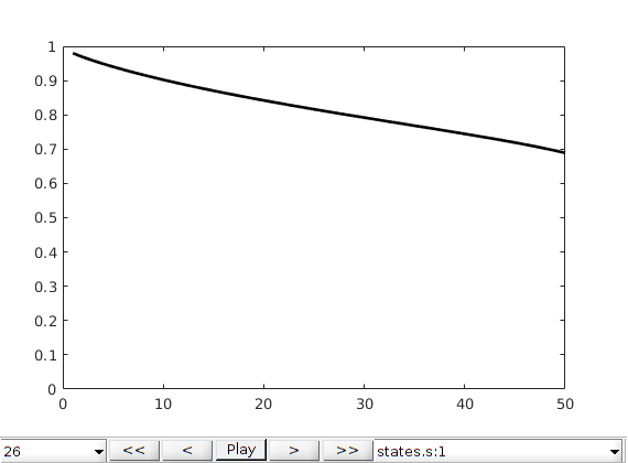
Repeat simulation with general solver¶

To use the general solver, we first need to set up a schedule that describes the time steps and the drive mechanisms (wells, boundary conditions, and source terms) that are active in each time step. In addition, one can specify various forms of time-step control. Here, however, we simply rely on the default setup

schedule = simpleSchedule(repmat(dT,1,n), 'bc', bc);
[~,sstates] = simulateScheduleAD(state0, model, schedule);

close all
plotToolbar(G, sstates, 'field', 's:1','lockCaxis',true),
caxis([0 1]), view(10,10)
colorbar

*****************************************************************
********** Starting simulation:    25 steps,   500 days *********
*****************************************************************
Preparing model for simulation...
Model ready for simulation...
Preparing schedule for simulation...
Schedule ready for simulation...
Validating initial state...
...

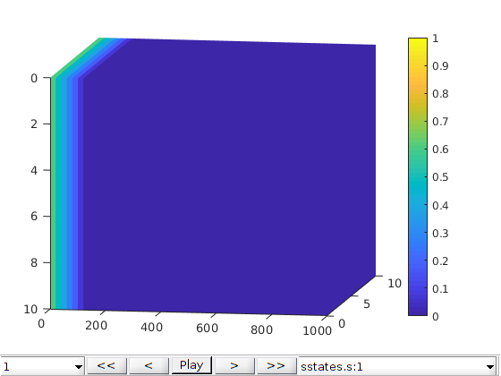
Repeat simulation with visualization¶

The general solver has a hook, that enables you to visualize the progress of the simulation (and stop it and continue running it in ‘debug’ mode).

close all
fn = getPlotAfterStep(state0, model, schedule, ...
    'plotWell', false, 'plotReservoir', true, 'field', 's:1', ...
    'lockCaxis',true, 'plot1d', true);

[~,sstates,report] = ...
   simulateScheduleAD(state0, model, schedule,'afterStepFn', fn);

*****************************************************************
********** Starting simulation:    25 steps,   500 days *********
*****************************************************************
Preparing model for simulation...
Model ready for simulation...
Preparing schedule for simulation...
Schedule ready for simulation...
Validating initial state...
...

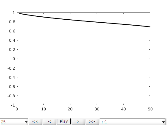
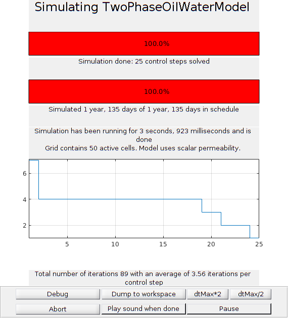
Repeat simulation with a storage handler¶

The solver also has a hook that enables you to control how the computed states are stored. To control the storage, we use a so-called storage handler, which behaves almost like a cell array, whose content can either be stored in memory, on disk, or both places. Here, we set it up to store on disk

handler = ResultHandler('writeToDisk', true, 'dataFolder', 'AD-BL1D');
simulateScheduleAD(state0, model, schedule, 'outputHandler', handler);
disp(handler)

*****************************************************************
********** Starting simulation:    25 steps,   500 days *********
*****************************************************************
Preparing model for simulation...
Model ready for simulation...
Preparing schedule for simulation...
Schedule ready for simulation...
Validating initial state...
...

The simulation above stored each state as a separate *.mat file in a subdirectory ‘AD-BL1D’ somewhere on a standard path relative to MRST’s root directory. The time steps can now be accessed in the usual way as if they were in memory. We can, for instance, pass the handler to the visualization GUI:

figure
plotToolbar(G, handler, 'field', 's:1','lockCaxis', true, 'plot1d', true);

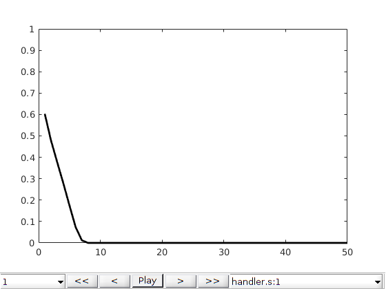
At a later stage, we can go back and retrieve the data from disk by constructing a new handler pointing to the same folder

clear handler

handler = ResultHandler('dataFolder', 'AD-BL1D');
m = handler.numelData();
states = cell(m, 1);
for i = 1:2:m
    states{i} = handler{i};
end

If we do not want to keep the data, they can be removed by a call to the reset function:

handler.resetData()

Copyright notice¶

<html>
% <p><font size="-1

Managing simulations: Restart, packed problems and more¶

Generated from demoPackedProblems.m

When using MRST to simulate larger or many problems, it is best to ensure that the results are stored to disk in a predictible manner. Otherwise, output from a long simulation may be lost if Matlab is closed for whatever reason.

mrstModule add ad-core ad-blackoil ad-props mrst-gui

Set up a simple problem with quadratic and linear relperm¶

We set up a simple 1D displacement problem for purposes of this demonstration. We create the same scenario with two different fluid models: A version with linear relative permeability and one with quadratic.

name = '1d';
G = cartGrid([100, 1], [1000, 1000]);
rock = makeRock(G, 0.1*darcy, 0.3);
G = computeGeometry(G);
fluid_1 = initSimpleADIFluid('mu', [1, 1]*centi*poise, 'n', [1, 1], 'phases', 'wo', 'rho', [1000, 500]);

model_1 = TwoPhaseOilWaterModel(G, rock, fluid_1);
time = 10*year;
irate = sum(model_1.operators.pv)/time;
W = [];
W = addWell(W, G, rock, 1, 'type', 'rate', 'val', irate, 'comp_i', [1, 0]);
W = addWell(W, G, rock, G.cells.num, 'type', 'bhp', 'val', 100*barsa, 'comp_i', [1, 0]);

dt = rampupTimesteps(time, time/100);
schedule = simpleSchedule(dt, 'W', W);

state0 = initResSol(G, 150*barsa, [0, 1]);

% Second fluid model
fluid_2 = initSimpleADIFluid('mu', [1, 1]*centi*poise, 'n', [2, 2], 'phases', 'wo', 'rho', [1000, 500]);
model_2 = TwoPhaseOilWaterModel(G, rock, fluid_2);

Define two simulations¶

We create two atomic packed simulation problems. This is similar to using simulateScheduleAD, with the addition of a few parameters describing the problem.

% Define base name for all problems in this script
BaseName = 'test_packed';
% Define linear flux
problem_1 = packSimulationProblem(state0, model_1, schedule, BaseName, ...
                                'Name', 'linear_relperm', ...
                                'Description', '1D displacement with linear flux');
% Define nonlinaer flux
problem_2 = packSimulationProblem(state0, model_2, schedule, BaseName, ...
                                'Name', 'quadratic_relperm', ...
                                'Description', '1D displacement with non-linear flux');

Run simulation¶

This will only simulate what is not yet simulated, and can restart aborted simulations in a seamless manner by using the ResultHandler class internally.

problems = {problem_1, problem_2};
[ok, status] = simulatePackedProblem(problems);

We can get output, just as if we simulated in the standard manner¶

[ws_1, states_1, reports_1] = getPackedSimulatorOutput(problem_1);
[ws_2, states_2, reports_2] = getPackedSimulatorOutput(problem_2);

For many packed problems, we can also get the data in a single call¶

[all_ws, all_states, all_reports, names, report_time] = getMultiplePackedSimulatorOutputs(problems);

Plot well results¶

plotWellSols(all_ws, report_time, 'DatasetNames', names, 'field', 'qWs', 'SelectedWells', 2);

Remove data (with prompts)¶

clearPackedSimulatorOutput(problems)

We can also launch simulations in the background¶

This is useful for running multiple cases. This functionality does not require any Matlab add-ons, since it creates an additional Matlab session which runs in the background. Please note that the additional sessions will terminate upon completion on error, but for larger cases this may take some time. You should not launch more sessions than your workstation can handle! First, remove data (without prompt before deletion)

learPackedSimulatorOutput(problems, 'prompt', false)
% Launch simulations
for i = 1:numel(problems)
    info = simulatePackedProblemBackground(problems{i}, 'verbose', true);
end
% Monitor the simulations running in the background
monitorBackgroundSimulations(problems);

% <html>
% <p><font size="-1

The use of regions: Different functions in different parts of the domain¶

Generated from differentRegionFunctionsExample.m

In many applications there is a need for varying functions in different parts of the domain. A typical example of this is the problem of varying rock types, where multiphase flow happens in a medium where the surface properties and porous structure varies significantly in different regions of the domain. In this example we demonstrate how to set up multiple rock types for relative permeability. The purpose of this example is to show the function interfaces used to have varying functions. The problem is not intended to be realistic.

mrstModule add ad-core ad-blackoil ad-props mrst-gui

Set up parameters¶

We create a small grid, with initially uniform fluid parameters.

dims = [20, 20];
G = cartGrid(dims, [1, 1]);
G = computeGeometry(G);
fluid = initSimpleADIFluid('phases', 'wo', 'rho', [100, 100],...
                            'cR', 1e-10/barsa, ...
                                           'mu', [1, 1]);

Computing normals, areas, and centroids...    Elapsed time is 0.000118 seconds.
Computing cell volumes and centroids...               Elapsed time is 0.000750 seconds.

Add multiple relative permeability functions¶

We create a quadratic and a linear relative-permeability relation as function handles of the saturation. We define the water and oil relative permeability to be equal as cell arrays. In doing so, the first entry corresponds to the first region and the second function to the second region and so on. We also create a cell-wise region indicator to map the two functions we have defined onto the grid. The exact mechanism for how we set up the region in the model can vary.

kr_1 = @(S) S.^2;
kr_2 = @(S) S;
fluid.krW = {kr_1, kr_2};
fluid.krO = {kr_1, kr_2};

rock = makeRock(G, 0.1*darcy, 0.3);
reg = 1 + double(G.cells.centroids(:, 2) > 0.5);

Plot the fluid regions and the corresponding relative permeability curves¶

We have a top and bottom part of the domain

figure;
subplot(1, 2, 1)
plotCellData(G, reg);
axis equal tight
colorbar('horiz')
colormap(lines(2));

subplot(1, 2, 2); hold on;
s = (0:0.05:1)';
nkr = numel(fluid.krW);
l = cell(1, nkr);
for i = 1:nkr
    k = fluid.krW{i};
    plot(s, k(s), 'linewidth', 2);
    l{i} = sprintf('Region %d', i);
end
legend(l, 'location', 'northwest');
xlabel('Saturation');
title('Relative permeability functions')

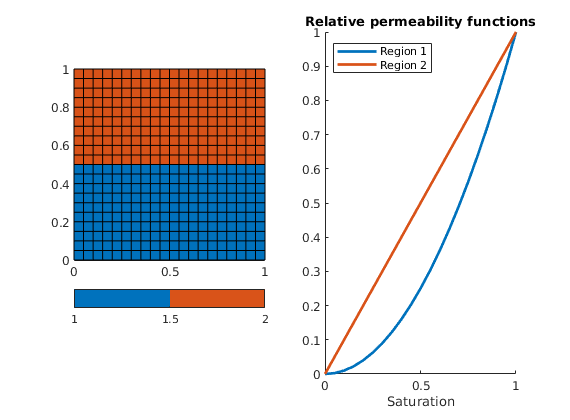
_images/differentRegionFunctionsExample_01.png

Set up simulation scenario¶

We inject 1 pore-volume over 100 days, from the left part of the domain to the right.

pv = poreVolume(G, rock);
time = 100*day;
irate = sum(pv)/time;
bc = [];
bc = fluxside(bc, G, 'Xmin', irate, 'sat', [1, 0]);
bc = pside(bc, G, 'XMax', 100*barsa, 'sat', [1, 0]);

state0 = initResSol(G, 100*barsa, [0, 1]);
schedule = simpleSchedule(rampupTimesteps(time, time/10), 'bc', bc);

Approach 1: Use different rock-types¶

We can set the rock.regions.saturation field to set up the different regions for the model. This is the default place the relative permeability and capillary pressure implementations will look for a region.

rock_reg = rock;
rock_reg.regions = struct('saturation', reg);
model = GenericBlackOilModel(G, rock_reg, fluid, 'gas', false);
[~, states] = simulateScheduleAD(state0, model, schedule);

figure;
plotToolbar(G, states, 'startPlayBack', true, 'field', 's:1')
title('Different regions (via rock)');

*****************************************************************
********** Starting simulation:    18 steps,   100 days *********
*****************************************************************
Preparing model for simulation...
Model ready for simulation...
Preparing schedule for simulation...
Schedule ready for simulation...
Validating initial state...
...

_images/differentRegionFunctionsExample_02.png

Approach 2: Directly modify the state functions¶

For a more fine-grained approach, we can manually update the RelativePermeability state function to have a new region. If a state function is using a function handle from the fluid in it’s implementation and it has a “regions” field set up, it will use that to evaluate the function. Since it is possible to swap out the StateFunctions to change the implementation of a single function, there are many ways to incorporate spatially varying functions.

model = GenericBlackOilModel(G, rock, fluid, 'gas', false);
model = model.validateModel();
model.FlowPropertyFunctions.RelativePermeability.regions = reg;

[~, states2] = simulateScheduleAD(state0, model, schedule);
figure;
plotToolbar(G, states2, 'startPlayBack', true, 'field', 's:1')
title('Different regions (via rock)');

*****************************************************************
********** Starting simulation:    18 steps,   100 days *********
*****************************************************************
Preparing model for simulation...
Model ready for simulation...
Preparing schedule for simulation...
Schedule ready for simulation...
Validating initial state...
...

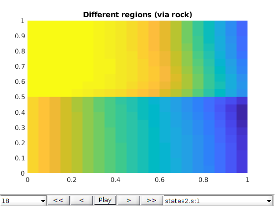
_images/differentRegionFunctionsExample_03.png

Approach 3: Use input files¶

We do not demonstrate this in this example, but if you build your model using inputs from the deckformat module, regions are automatically set up if present.

<html>
% <p><font size="-1

Demonstrate Interactive Plotting of Fluid Properties for AD-solvers¶

Generated from fluidInspectionExample.m

The AD-OO framework can interactively visualize the fluid model of a ReservoirModel instance. Once active, the user can interactively explore the different fluid properties (viscosities, relative permeabilities, densities) as functions of saturation and pressure. Load the blackoil module and others to create test data.

mrstModule add ad-blackoil ad-core ad-props deckformat

Inspect the SPE1 fluid model¶

The SPE1 fluid model is a three-phase blackoil model with solution gas. For more information, as well as a simulation example, see the SPE1 blackoil tutorial. We use a setup routine to get a ReservoirModel subclass, and pass it to inspectFluidModel. Note that in this specific case, the tables for undersaturated values can lead to negative or discontinuous values for certain high pressure values. This is not always easy to see directly from the tables, but by using the fluid inspector it is straightforward.

[G, rock, fluid, deck] = setupSPE1();
spe1 = selectModelFromDeck(G, rock, fluid, deck);

inspectFluidModel(spe1, 'pressureRange', (0:10:500)*barsa)

No converter needed in section 'REGIONS'.
No converter needed in section 'SUMMARY'.
Adding 200 artificial cells at top/bottom

Processing regular i-faces
 Found 550 new regular faces
Elapsed time is 0.001499 seconds.

...

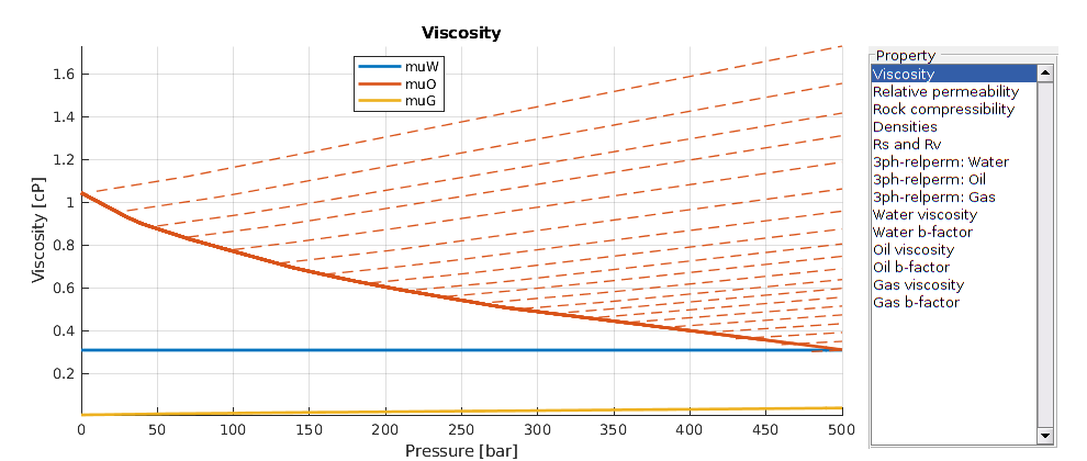
Inspect the SPE9 fluid model¶

Another standard black-oil test case is the SPE9 model. For more information about this test case, see the SPE9 black-oil tutorial. Of particular interest in this case is the non-zero capillary pressure, and the highly irregular relative permeability curves.

[G, rock, fluid, deck] = setupSPE9();
spe9 = selectModelFromDeck(G, rock, fluid, deck);

inspectFluidModel(spe9)

No converter needed in section 'REGIONS'.
No converter needed in section 'SUMMARY'.
Adding 1200 artificial cells at top/bottom

Processing regular i-faces
 Found 10625 new regular faces
Elapsed time is 0.004735 seconds.

...

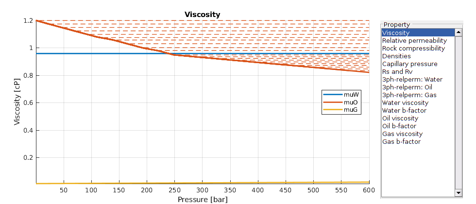
Set up a two-phase oil-water fluid and inspect it¶

We can use the inspection utility to get a better understanding of how the fluid model changes when we adjust parameters. In this case, we set up a simple two-phase, oil-water model and add in other relative permeability curves with different residual values and Corey exponents. Feel free to modify the parameters and look at how the values change.

fluid = initSimpleADIFluid('phases', 'WO', ...
                           'rho', [1000, 700], ...
                           'cR',  1e-8/barsa, ...
                           'c',   [0, 1e-4/barsa]);
srw = 0.2;
sro = 0.3;

% Fluid relative permeabilities (use name convention from SWOF keyword)
fluid.krW  = coreyPhaseRelpermAD(2, srw, 1, srw + sro);
fluid.krOW = coreyPhaseRelpermAD(4, sro, 1, srw + sro);

model_ow = TwoPhaseOilWaterModel([], [], fluid);

% Inspect model, and specify pressure range of interest
inspectFluidModel(model_ow, 'pressureRange', (250:10:500)*barsa);

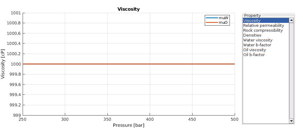
Copyright notice¶

<html>
% <p><font size="-1

Introduction to StateFunctions for the AD-OO framework¶

Generated from stateFunctionTutorial.m

The StateFunction class, together with the StateFunctionGrouping class, is the main mechanism for evaluating properties during a AD-OO simulation. These functions act directly on the “state” object and fully support automatic differentiation, lazy evaluation and different regions.

mrstModule add ad-core ad-blackoil deckformat ad-props

Create a black-oil test model¶

We set up the SPE1 model, a black-oil model with disgas (but no vapoil).

pth = getDatasetPath('spe1');
fn  = fullfile(pth, 'BENCH_SPE1.DATA');
[state0, model, schedule, nonlinear] = initEclipseProblemAD(fn);

No converter needed in section 'REGIONS'.
No converter needed in section 'SUMMARY'.
Adding 200 artificial cells at top/bottom

Processing regular i-faces
 Found 550 new regular faces
Elapsed time is 0.000880 seconds.

...

Validate model to set up defaults¶

State functions are set up at the start of a simulation, with reasonable defaults given. Here, we manually call validateModel to invoke these defaults.

model = model.validateModel();
% We can now get the groupings belonging to this model
groups = model.getStateFunctionGroupings();

Test the evaluation¶

Each grouping is a collection of one or more StateFunctions, which can depend on each other, or the state of the physical system itself. Dependencies between these are automatically handled during simulations. For instance, let us get the mobility of the initial state. We then plot the oil mobility on the grid.

% We can get this with getProp, just as we would with the pressure or
% saturations which are stored directly in the state. Normally, we do not
% have to think too hard about where exactly a property is defined, since
% the framework can figure it out for us.
mobility = model.getProp(state0, 'Mobility');
% Alternatively, we could invoke the FlowPropertyFunctions grouping's get
% function to the same effect.
mob = model.FlowPropertyFunctions.get(model, state0, 'Mobility');

figure;
plotCellData(model.G, mobility{2});
title('Initial oil mobility')
view(30, 30);
colorbar

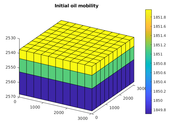
We can also initialize AD-variables in state to get derivatives¶

Initialize pressure as a AD-variable

stateAD = state0;
stateAD.pressure = initVariablesADI(state0.pressure);
% Outputs are now ADI, with differentiation with respect to pressure
mobAD = model.FlowPropertyFunctions.get(model, stateAD, 'Mobility');
disp(mobAD)

[1×1 ADI]    [1×1 ADI]    [1×1 ADI]

Show a state function grouping¶

We can inspect the FlowPropertyFunctions directly. The FlowPropertyFunctions consist of the basic properties required for flow in MRST. Additional properties can be added dynamically to the class instance itself.

disp(model.FlowPropertyFunctions)

<a href="matlab:helpPopup FlowPropertyFunctions">FlowPropertyFunctions</a> (<a href="matlab:edit FlowPropertyFunctions.m">edit</a>) state function grouping instance.

  Intrinsic properties (Class properties for FlowPropertyFunctions, always present):

        CapillaryPressure: <a href="matlab:helpPopup BlackOilCapillaryPressure">BlackOilCapillaryPressure</a> (<a href="matlab:edit BlackOilCapillaryPressure.m">edit</a>)
        ComponentMobility: <a href="matlab:helpPopup ComponentMobility">ComponentMobility</a> (<a href="matlab:edit ComponentMobility.m">edit</a>)
    ComponentPhaseDensity: <a href="matlab:helpPopup ComponentPhaseDensity">ComponentPhaseDensity</a> (<a href="matlab:edit ComponentPhaseDensity.m">edit</a>)
       ComponentPhaseMass: <a href="matlab:helpPopup ComponentPhaseMass">ComponentPhaseMass</a> (<a href="matlab:edit ComponentPhaseMass.m">edit</a>)
...

Plot dependencies¶

Generally, only a few values are needed to assemble the final linearized equation. Many other functions may be required to get intermediate results, however. For instance, capillary pressure does not occur directly in the flow equations, but standard functions for density, phase pressures and viscosity can depend strongly on the capillary pressure between phases. We can plot the dependency graph of all the state function groupings in order to understand the relationships between the different functions.

for i = 1:numel(groups)
    figure;
    plotStateFunctionGroupings(groups{i})
    title(class(groups{i}));
end

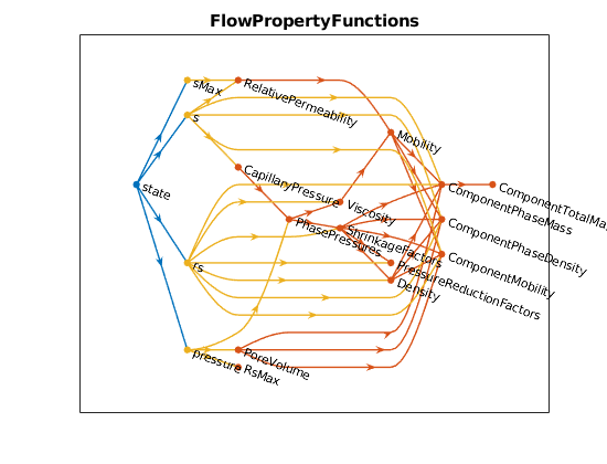
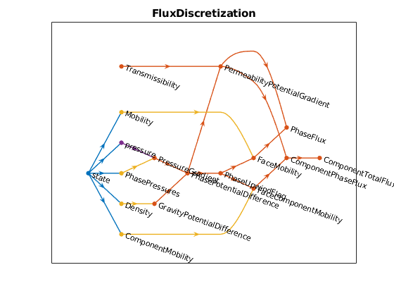
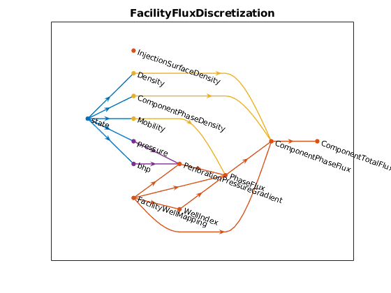
Plot a specific dependency¶

Plot all dependencies for the mobility we just evaluated

figure(1); clf
plotStateFunctionGroupings(model.FlowPropertyFunctions, 'Stop', 'Mobility')
title('All dependencies required to evaluate mobility')

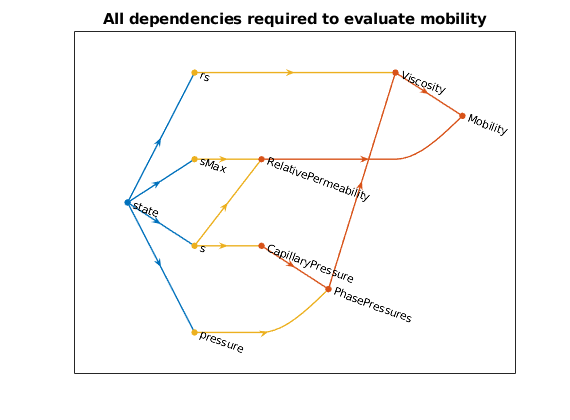
Plot all dependencies of a property¶

Let’s see all properties which directly or indirectly depend on on the pressure in the state

figure(1); clf
plotStateFunctionGroupings(model.FlowPropertyFunctions, 'Start', 'pressure')
title('Flow properties that depend on pressure')

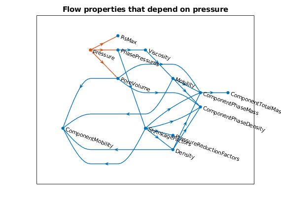
Plot everything which either depends upon a property, or uses that property¶

Let’s see all properties which directly or indirectly depend on on the pressure in the state

figure(1); clf
plotStateFunctionGroupings(model.FlowPropertyFunctions, 'Center', 'Mobility')
title('Upstream and downstream mobility dependencies');

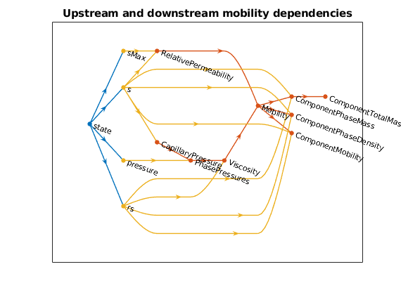
We can combine graphs¶

Here, we plot all the flow properties together with the discretization of the flux, which depends on many of these properties.

df = get(0, 'DefaultFigurePosition');
figure('Position', df.*[1, 1, 2, 2]);
tmp = {model.FlowPropertyFunctions, model.FluxDiscretization};
plotStateFunctionGroupings(tmp);
title('Flow properties + flow discretization')

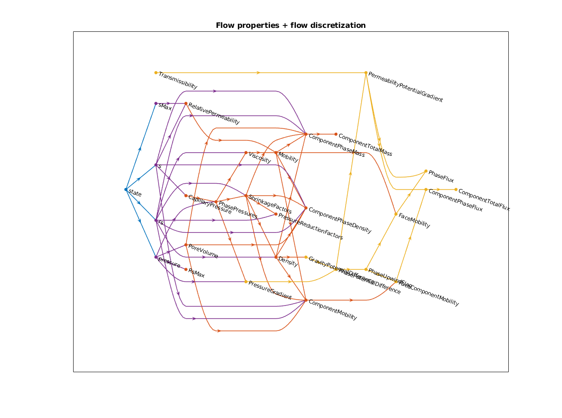
Create a compositional model and visualize the property graphs¶

We create a compositional model, which has a few major differences from the black-oil model: Note the addition of equation-of-state properties such as fugacity or phase compressibility factors. In addition, the relationship between the ShrinkageFactors and Density

rstModule add compositional
eos = getCompositionalFluidCase('simple');
cmodel = GenericNaturalVariablesModel(model.G, model.rock, model.fluid, eos, 'water', true);
cmodel = cmodel.validateModel();

clf;
plotStateFunctionGroupings(cmodel.FlowPropertyFunctions);

% <html>
% <p><font size="-1

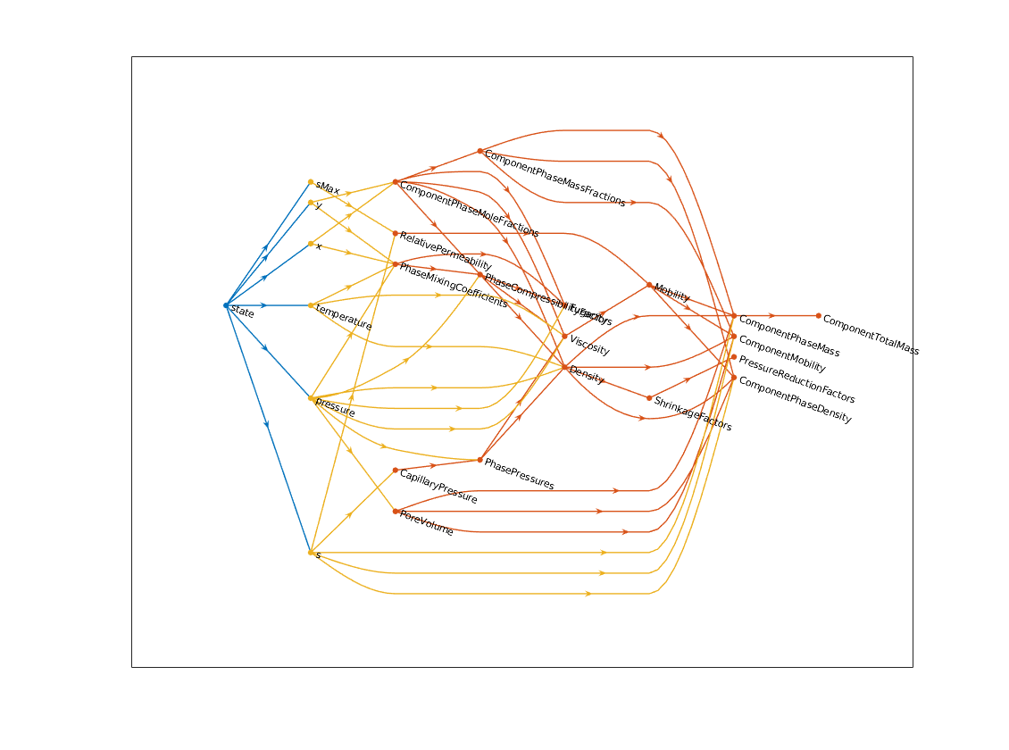
mrstModule add ad-core ad-blackoil ad-props

Set up scenario¶

Generated from wenoExampleAD.m

dims = [50, 50];
pdims = [100, 100];

G = cartGrid(dims, pdims);
G = computeGeometry(G);

rock = makeRock(G, 0.1*darcy, 0.3);
fluid = initSimpleADIFluid('n', [1, 1], 'mu', [1, 1]*centi*poise, 'rho', [100, 100], 'phases', 'wo');
model = GenericBlackOilModel(G, rock, fluid, ...
                        'water', true, 'oil', true, 'gas', false);
time = 1*year;
irate = 2*sum(model.operators.pv)/time;

W = [];
W = addWell(W, G, rock, 1, 'comp_i', [1, 0], 'val', irate, 'type', 'rate');
W = addWell(W, G, rock, G.cells.num, 'comp_i', [1, 0], 'val', 50*barsa, 'type', 'bhp');

n = 300;
dt = repmat(time/n, n, 1);
schedule = simpleSchedule(dt, 'W', W);

state0 = initResSol(G, 100*barsa, [0, 1]);

Computing normals, areas, and centroids...    Elapsed time is 0.001207 seconds.
Computing cell volumes and centroids...               Elapsed time is 0.002973 seconds.
Defaulting reference depth to top of formation for well W1. Please specify 'refDepth' optional argument to 'addWell' if you require bhp at a specific depth.
Defaulting reference depth to top of formation for well W2. Please specify 'refDepth' optional argument to 'addWell' if you require bhp at a specific depth.

Simulate base case¶

[ws, states, report] = simulateScheduleAD(state0, model, schedule);

*****************************************************************
********** Starting simulation:   300 steps,   365 days *********
*****************************************************************
Preparing model for simulation...
Model ready for simulation...
Preparing schedule for simulation...
Schedule ready for simulation...
Validating initial state...
...

Set up a WENO discretization¶

model_weno = model;
weno = WENOUpwindDiscretization(model_weno);

Getting supports.
of 2500...
of 2500...
of 2500...
of 2500...
of 2500...
of 2500...
of 2500...
...

Override the component discretization with a WENO scheme¶

model_weno = model_weno.validateModel();
props = model_weno.FluxDiscretization;
disp(props)
props = props.setStateFunction('FaceMobility', FaceMobility(model_weno, weno));
props = props.setStateFunction('FaceComponentMobility', FaceComponentMobility(model_weno, weno));
model_weno.FluxDiscretization = props;

[ws_weno, states_weno, report_weno] = simulateScheduleAD(state0, model_weno, schedule);

<a href="matlab:helpPopup FluxDiscretization">FluxDiscretization</a> (<a href="matlab:edit FluxDiscretization.m">edit</a>) state function grouping instance.

  Intrinsic properties (Class properties for FluxDiscretization, always present):

            ComponentPhaseFlux: <a href="matlab:helpPopup ComponentPhaseFlux">ComponentPhaseFlux</a> (<a href="matlab:edit ComponentPhaseFlux.m">edit</a>)
            ComponentTotalFlux: <a href="matlab:helpPopup ComponentTotalFlux">ComponentTotalFlux</a> (<a href="matlab:edit ComponentTotalFlux.m">edit</a>)
         FaceComponentMobility: <a href="matlab:helpPopup FaceComponentMobility">FaceComponentMobility</a> (<a href="matlab:edit FaceComponentMobility.m">edit</a>)
    GravityPotentialDifference: <a href="matlab:helpPopup GravityPotentialDifference">GravityPotentialDifference</a> (<a href="matlab:edit GravityPotentialDifference.m">edit</a>)
...

model_e = model.validateModel();
fd = model_e.FluxDiscretization;
fd = fd.setFlowStateBuilder(AdaptiveImplicitFlowStateBuilder('initialStep', 0.02*day, 'verbose', true));
model_e.FluxDiscretization = fd;
[ws_e, states_e, report_e] = simulateScheduleAD(state0, model_e, schedule);

*****************************************************************
********** Starting simulation:   300 steps,   365 days *********
*****************************************************************
Preparing model for simulation...
Model ready for simulation...
Preparing schedule for simulation...
Schedule ready for simulation...
Validating initial state...
...

model_weno_expl = model_weno;
fd = model_weno_expl.FluxDiscretization;
fd = fd.setFlowStateBuilder(AdaptiveImplicitFlowStateBuilder('initialStep', 0.02*day, 'verbose', true));
model_weno_expl.FluxDiscretization = fd;
[ws_weno_ex, states_weno_ex, report_weno_ex] = simulateScheduleAD(state0, model_weno_expl, schedule);

*****************************************************************
********** Starting simulation:   300 steps,   365 days *********
*****************************************************************
Preparing model for simulation...
Model ready for simulation...
Preparing schedule for simulation...
Schedule ready for simulation...
Validating initial state...
...

Plot saturations¶

G.cells.sortedCellNodes = getSortedCellNodes(G);
for i = 1:numel(states)
    figure(1); clf;
    subplot(2, 2, 1)
    plotCellData(G, states{i}.s(:, 1), 'edgecolor', 'none');
    axis equal tight
    title('FIM SPU');
    subplot(2, 2, 2)
    plotCellData(G, states_weno{i}.s(:, 1), 'edgecolor', 'none');
    axis equal tight
    title('FIM WENO')
    subplot(2, 2, 3)
    plotCellData(G, states_e{i}.s(:, 1), 'edgecolor', 'none');
    title('AIM SPU')
    axis equal tight

    subplot(2, 2, 4)
    plotCellData(G, states_weno_ex{i}.s(:, 1), 'edgecolor', 'none');
    title('AIM WENO')
    axis equal tight
end

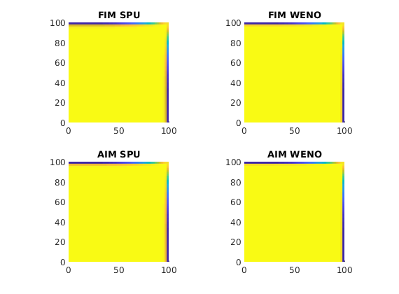
Plot wells¶

lotWellSols({ws, ws_e, ws_weno, ws_weno_ex}, report.SimulationTime, 'datasetnames', {'FIM-SPU', 'AIM-SPU', 'FIM-WENO', 'AIM-WENO'}, 'field', 'qWs', 'SelectedWells', 2)

% <html>
% <p><font size="-1

ad-core: Automatic Differentiation Core¶

Models¶

Base classes¶

Facility and wells¶

Simulators¶

Solvers¶

Time-step selection¶

Model upscaling¶

Plotting¶

Automatic differentation backends¶

Utilities¶

Examples¶

Classic Buckley-Leverett Problem: 1D Horizontal Displacement¶

Set up model¶

Simulate 1 PVI using a manual loop¶

Plot the result¶

Repeat simulation with general solver¶

Repeat simulation with visualization¶

Repeat simulation with a storage handler¶

Copyright notice¶

Managing simulations: Restart, packed problems and more¶

Set up a simple problem with quadratic and linear relperm¶

Define two simulations¶

Run simulation¶

We can get output, just as if we simulated in the standard manner¶

For many packed problems, we can also get the data in a single call¶

Plot well results¶

Remove data (with prompts)¶

We can also launch simulations in the background¶

The use of regions: Different functions in different parts of the domain¶

Set up parameters¶

Add multiple relative permeability functions¶

Plot the fluid regions and the corresponding relative permeability curves¶

Set up simulation scenario¶

Approach 1: Use different rock-types¶

Approach 2: Directly modify the state functions¶

Approach 3: Use input files¶

Demonstrate Interactive Plotting of Fluid Properties for AD-solvers¶

Inspect the SPE1 fluid model¶

Inspect the SPE9 fluid model¶

Set up a two-phase oil-water fluid and inspect it¶

Copyright notice¶

Introduction to StateFunctions for the AD-OO framework¶

Create a black-oil test model¶

Validate model to set up defaults¶

Test the evaluation¶

We can also initialize AD-variables in state to get derivatives¶

Show a state function grouping¶

Plot dependencies¶

Plot a specific dependency¶

Plot all dependencies of a property¶

Plot everything which either depends upon a property, or uses that property¶

We can combine graphs¶

Create a compositional model and visualize the property graphs¶

Set up scenario¶

Simulate base case¶

Set up a WENO discretization¶

Override the component discretization with a WENO scheme¶

Plot saturations¶

Plot wells¶

`ad-core`: Automatic Differentiation Core¶