ad-blackoil: Black-oil solvers
Models and examples that extend the MRST AD-OO framework found in the ad-core module to black-oil problems. More specifically, the module adds additional models that implement the black-oil equations for multiphase, miscible, compressible flow. Included in the module are also a wide variety of examples validating the solvers against a commercial simulator on standard test cases.
The module includes single-phase, two-phase and three-phase solvers. The three-phase solvers has optional support for problems where gas can dissolve into oil (Rs) and/or oil can vaporize into the gas phase (Rv). The solvers support source terms, boundary conditions and complex wells with changing controls, production limits and multiple segments. Standard benchmark cases (SPE1, SPE9) are included together with comparison results from a commercial simulator.
Models
Base classes
-
Contents¶ MODELS
- Files
- AquiferBlackOilModel - GenericBlackOilModel - ThreePhaseBlackOilModel - Three phase with optional dissolved gas and vaporized oil TwoPhaseOilWaterModel - Two phase oil/water system without dissolution WaterModel - Single phase water model. WaterThermalModel - Single phase water model with thermal effects. Should be considered
-
class
ThreePhaseBlackOilModel(G, rock, fluid, varargin)¶ Bases:
ReservoirModelThree phase with optional dissolved gas and vaporized oil
-
getPrimaryVariables(model, state)¶ Get primary variables from state, before a possible initialization as AD.
-
getScalingFactorsCPR(model, problem, names, solver)¶ Get approximate, impes-like pressure scaling factors
-
validateModel(model, varargin)¶ Validate model.
-
validateState(model, state)¶ Check parent class
-
disgas= None¶ Flag deciding if oil can be vaporized into the gas phase
-
drsMaxRel= None¶ Maximum absolute Rs/Rv increment
-
vapoil= None¶ Maximum relative Rs/Rv increment
-
-
class
TwoPhaseOilWaterModel(G, rock, fluid, varargin)¶ Bases:
ThreePhaseBlackOilModelTwo phase oil/water system without dissolution
-
class
WaterModel(G, rock, fluid, varargin)¶ Bases:
ReservoirModelSingle phase water model.
-
class
WaterThermalModel(G, rock, fluid, varargin)¶ Bases:
WaterModelSingle phase water model with thermal effects. Should be considered experimental and intentionally undocumented, as this feature is subject to change in the future.
-
insertWellEquations(model, eqs, names, types, wellSol0, wellSol, wellVars, wellMap, p, mob, rho, hW, components, dt, opt)¶ Utility function for setting up the well equations and adding source terms for black-oil like models. Note that this currently assumes that the first nPh equations are the conservation equations, according to the canonical MRST W-O-G ordering,
-
Utilities
-
Contents¶ UTILS
- Files
- assignWellValuesFromControl - Assign wellSol values when values are set as controls calculateHydrocarbonsFromStatusBO - Compute solution variables for the gas/oil/rs/rv-variable in black-oil computeAquiferFluxes - Undocumented Utility Function computeFlashBlackOil - Compute flash for a black-oil model with disgas/vapoil computeInitAquifer - Undocumented Utility Function equationsBlackOil - Generate linearized problem for the black-oil equations equationsOilWater - Generate linearized problem for the two-phase oil-water model equationsWater - Generate linearized problem for the single-phase water model equationsWaterThermal - Get linearized problem for single phase water system with black oil-style getbG_BO - Utility function for evaluating the reciprocal gas formation volume getbO_BO - Utility function for evaluating the reciprocal oil formation volume getCapillaryPressureBO - Compute oil-water and oil-gas capillary pressures getCellStatusVO - Get status flags for each cell in a black-oil model getDeckEGG - Get the parsed deck for the EGG model getFluxAndPropsGas_BO - Get flux and properties for the gas phase for a black-oil problem getFluxAndPropsOil_BO - Get flux and properties for the oil phase for a black-oil problem getFluxAndPropsWater_BO - Get flux and properties for the water phase for a black-oil problem getPolymerShearMultiplier - Compute the flux multiplier due to polymer shear thinning/thickening getWellPolymer - Undocumented Utility Function updateStateBlackOilGeneric - Generic update function for blackoil-like models
-
assignWellValuesFromControl(model, wellSol, W, wi, oi, gi)¶ Assign wellSol values when values are set as controls
Synopsis:
wellSol = assignWellValuesFromControl(model, wellSol, W, wi, oi, gi)
Description:
Well rates and pressures can be both controls and solution variables, depending on the problem. For a subset of possible well controls, this function explicitly assigns the values to the wellSol.
Parameters: - model – ReservoirModel-derived subclass.
- wellSol – wellSol to be updated.
- W – Well struct used to create wellSol.
- oi, gi (wi,) – Indices for water, oil and gas respectively in the .compi field of the well.
Returns: wellSol – Updated wellSol where fields corresponding to assigned controls have been modified.
See also
WellModel
-
calculateHydrocarbonsFromStatusBO(fluid, status, sO, x, rs, rv, pressure, disgas, vapoil)¶ Compute solution variables for the gas/oil/rs/rv-variable in black-oil
Synopsis:
[sG, rs, rv, rsSat, rvSat] = ...
calculateHydrocarbonsFromStatusBO(model, status, sO, x, rs, rv, pressure)
Description:
The ThreePhaseBlackOil model has a single unknown that represents either gas, oil, oil in gas (rs) and gas in oil (rv) on a cell-by-cell basis. The purpose of this function is to easily compute the different quantities from the “x”-variable and other properties, with correct derivatives if any of them are AD-variables.
Parameters: - model – ThreePhaseBlackOilModel-derived class. Determines if vapoil/disgas is being used and contains the fluid model.
- status – Status flag as defined by “getCellStatusVO”
- sO – The tentative oil saturation.
- x – Variable that is to be decomposed into sG, sO, rs, rv, …
- rv (rs,) – Dissolved gas, vaporized oil
- pressure – Reservoir oil pressure
- disgas – true if dissolved gas should be taken into account
- vapoil – true if vaporized oil should be taken into account
Keyword Arguments: ‘field’
RETURNS:
See also
equationsBlackOil, getCellStatusVO
-
computeAquiferFluxes(model, state, dt)¶ Undocumented Utility Function
-
computeFlashBlackOil(state, state0, model, status)¶ Compute flash for a black-oil model with disgas/vapoil
Synopsis:
state = computeFlashBlackOil(state, state0, model, status)
Description:
Compute flash to ensure that dissolved properties are within physically reasonable values, and simultanously avoid that properties go far beyond the saturated zone when they were initially unsaturated and vice versa.
Parameters: - state – State where saturations, rs, rv have been updated due to a Newton-step.
- state0 – State from before the linearized update.
- model – The ThreePhaseBlackOil derived model used to compute the update.
- status – Status flags from getCellStatusVO, applied to state0.
Returns: state – Updated state where saturations and values are chopped near phase transitions.
Note
Be mindful of the definition of state0. It is not necessarily the state at the previous timestep, but rather the state at the previous nonlinear iteration!
-
computeInitAquifer(model, initState, initaqvolumes)¶ Undocumented Utility Function
-
equationsBlackOil(state0, state, model, dt, drivingForces, varargin)¶ Generate linearized problem for the black-oil equations
Synopsis:
[problem, state] = equationsBlackOil(state0, state, model, dt, drivingForces)
Description:
This is the core function of the black-oil solver. This function assembles the residual equations for the conservation of water, oil and gas, as well as required well equations. By default, Jacobians are also provided by the use of automatic differentiation.
Oil can be vaporized into the gas phase if the model has the vapoil property enabled. Analogously, if the disgas property is enabled, gas is allowed to dissolve into the oil phase. Note that the fluid functions change depending on vapoil/disgas being active and may have to be updated when the property is changed in order to run a successful simulation.
Parameters: - state0 – Reservoir state at the previous timestep. Assumed to have physically reasonable values.
- state – State at the current nonlinear iteration. The values do not need to be physically reasonable.
- model – ThreePhaseBlackOilModel-derived class. Typically, equationsBlackOil will be called from the class getEquations member function.
- dt – Scalar timestep in seconds.
- drivingForces – Struct with fields: * W for wells. Can be empty for no wells. * bc for boundary conditions. Can be empty for no bc. * src for source terms. Can be empty for no sources.
Keyword Arguments: - ‘Verbose’ – Extra output if requested.
- ‘reverseMode’ – Boolean indicating if we are in reverse mode, i.e. solving the adjoint equations. Defaults to false.
- ‘resOnly’ – Only assemble residual equations, do not assemble the Jacobians. Can save some assembly time if only the values are required.
- ‘iterations’ – Nonlinear iteration number. Special logic happens in the wells if it is the first iteration.
Returns: - problem – LinearizedProblemAD class instance, containing the water, oil and gas conservation equations, as well as well equations specified by the FacilityModel class.
- state – Updated state. Primarily returned to handle changing well controls from the well model.
See also
equationsOilWater, ThreePhaseBlackOilModel
-
equationsOilWater(state0, state, model, dt, drivingForces, varargin)¶ Generate linearized problem for the two-phase oil-water model
Synopsis:
[problem, state] = equationsOilWater(state0, state, model, dt, drivingForces)
Description:
This is the core function of the two-phase oil-water solver. This function assembles the residual equations for the conservation of water and oil as well as required well equations. By default, Jacobians are also provided by the use of automatic differentiation.
Parameters: - state0 – Reservoir state at the previous timestep. Assumed to have physically reasonable values.
- state – State at the current nonlinear iteration. The values do not need to be physically reasonable.
- model – TwoPhaseOilWaterModel-derived class. Typically, equationsOilWater will be called from the class getEquations member function.
- dt – Scalar timestep in seconds.
- drivingForces – Struct with fields: * W for wells. Can be empty for no wells. * bc for boundary conditions. Can be empty for no bc. * src for source terms. Can be empty for no sources.
Keyword Arguments: - ‘Verbose’ – Extra output if requested.
- ‘reverseMode’ – Boolean indicating if we are in reverse mode, i.e. solving the adjoint equations. Defaults to false.
- ‘resOnly’ – Only assemble residual equations, do not assemble the Jacobians. Can save some assembly time if only the values are required.
- ‘iterations’ – Nonlinear iteration number. Special logic happens in the wells if it is the first iteration.
Returns: - problem – LinearizedProblemAD class instance, containing the water and oil conservation equations, as well as well equations specified by the WellModel class.
- state – Updated state. Primarily returned to handle changing well controls from the well model.
See also
equationsBlackOil, TwoPhaseOilWaterModel
-
equationsWater(state0, state, model, dt, drivingForces, varargin)¶ Generate linearized problem for the single-phase water model
Synopsis:
[problem, state] = equationsWater(state0, state, model, dt, drivingForces)
Description:
This is the core function of the single-phase water solver with black-oil style properties. This function assembles the residual equations for the conservation of water and oil as well as required well equations. By default, Jacobians are also provided by the use of automatic differentiation.
Parameters: - state0 – Reservoir state at the previous timestep. Assumed to have physically reasonable values.
- state – State at the current nonlinear iteration. The values do not need to be physically reasonable.
- model – WaterModel-derived class. Typically, equationsWater will be called from the class getEquations member function.
- dt – Scalar timestep in seconds.
- drivingForces – Struct with fields: * W for wells. Can be empty for no wells. * bc for boundary conditions. Can be empty for no bc. * src for source terms. Can be empty for no sources.
Keyword Arguments: - ‘Verbose’ – Extra output if requested.
- ‘reverseMode’ – Boolean indicating if we are in reverse mode, i.e. solving the adjoint equations. Defaults to false.
- ‘resOnly’ – Only assemble residual equations, do not assemble the Jacobians. Can save some assembly time if only the values are required.
- ‘iterations’ – Nonlinear iteration number. Special logic happens in the wells if it is the first iteration.
Returns: - problem – LinearizedProblemAD class instance, containing the equation for the water pressure, as well as well equations specified by the WellModel class.
- state – Updated state. Primarily returned to handle changing well controls from the well model.
See also
equationsBlackOil, ThreePhaseBlackOilModel
-
equationsWaterThermal(state0, state, model, dt, drivingForces, varargin)¶ Get linearized problem for single phase water system with black oil-style properties
-
getCapillaryPressureBO(fluid, sW, sG)¶ Compute oil-water and oil-gas capillary pressures
Synopsis:
[pcOW, pcOG] = getCapillaryPressureBO(f, sW, sG)
Description:
Compute the capillary pressures relative to the oil pressure
Parameters: - fluid – AD fluid model, from for example initDeckADIFluid or initSimpleADIFluid.
- sW – Water saturation. Used to evaluate the water-oil capillary pressure.
- sG – Gas saturation. Used to evaluate the oil-gas capillary pressure.
Returns: - pcOW – Pressure difference between the oil and water pressures. The water phase pressure can be computed as pW = pO - pcOW;
- pcOG – Pressure difference between the oil and gas pressures. The water phase pressure can be computed as pG = pO + pcOG;
Note
Mind the different sign for the computation of the phase pressures above!
-
getCellStatusVO(sO, sW, sG, varargin)¶ Get status flags for each cell in a black-oil model
Synopsis:
st = getCellStatusVO(model, state, sO, sW, sG)
Description:
Get the status flags for the number of phases present.
Parameters: - sO – Oil saturation. One value per cell in the simulation grid.
- sW – Water saturation. One value per cell in the simulation grid.
- sG – Gas saturation. One value per cell in the simulation grid.
Keyword Arguments: - status – status that can be provided fom the state for which the status flags are to be computed.
- vapoil – true if there can be vaporized oil
- disgas – true if there can be dissolved gas
Returns: st –
- Cell array with three columns with one entry per cell. The
interpretation of each flag:
Col 1: A cell is flagged as true if oil is present, but gas is not present. Col 2: A cell is flagged as true if gas is present, but oil is not present. Col 3: A cell is flagged as true if both gas and oil are present and true three-phase flow is occuring.
See also
ThreePhaseBlackOilModel
-
getDeckEGG(varargin)¶ Get the parsed deck for the EGG model
-
getFluxAndPropsGas_BO(model, pO, sG, krG, T, gdz, rv, isSat)¶ Get flux and properties for the gas phase for a black-oil problem
Synopsis:
[vG, bG, mobG, rhoG, pG, upcg, dpG] = ...
   getFluxAndPropsOil_BO(model, pO, sG, krG, T, gdz, rv, isSat)
Description:
Utility function for evaluating mobilities, densities and fluxes for the gas phase in the black-oil (BO)-model
Parameters: - model – ThreePhaseBlackOil or derived subclass instance
- p – Oil phase pressure. One value per cell in simulation grid.
- sG – Gas phase saturation. One value per cell in simulation grid.
- krG – Gas phase relative permeability, possibly evaluated some three-phase relperm function. One value per cell in simulation grid.
- T – Transmissibility for the internal interfaces.
- gdz – Let dz be the gradient of the cell depths, on each interface.
- gdz is the dot product of the dz with the gravity vector of the (Then) –
- See getGravityGradient for more information. (model.) –
- rv – Amount of oil vaporized into the gas phase. Use to evaluate the viscosity and density. One value per cell in simulation grid.
- isSat – Boolean indicator if the gas in the cell is saturated with oil.
- indicates that the maximum vaporized gas is present inside the gas (True) –
- in the cell, and that we need to look at the saturated tables (phase) –
- evaluating rv (when) – dependent properties. One value per cell in
- grid. (simulation) –
Returns: - vG – Gas flux, at reservoir conditions, at each interface.
- bG – Gas reciprocal formation volume factors. One value per cell in simulation grid.
- rhoG – Gas density in each cell.
- pG – Gas phase pressure. One value per cell in simulation grid. Pressure will be different from the oil pressure if capillary pressure is present in the model.
- upcg – Upwind indicators for the gas phase. One value per interface.
- dpG – Phase pressure differential for each interface. Was used to evaluate the phase flux.
See also
getFluxAndPropsOil_BO, getFluxAndPropsWater_BO
-
getFluxAndPropsOil_BO(model, p, sO, krO, T, gdz, rs, isSat)¶ Get flux and properties for the oil phase for a black-oil problem
Synopsis:
[vO, bO, mobO, rhoO, p, upco, dpO] = ...
   getFluxAndPropsOil_BO(model, p, sO, krO, T, gdz, rs, isSat)
Description:
Utility function for evaluating mobilities, densities and fluxes for the oil phase in the black-oil (BO)-model
Parameters: - model – ThreePhaseBlackOil or derived subclass instance
- p – Oil phase pressure. One value per cell in simulation grid.
- sO – Oil phase saturation. One value per cell in simulation grid.
- krO – Oil phase relative permeability, possibly evaluated some three-phase relperm function. One value per cell in simulation grid.
- T – Transmissibility for the internal interfaces.
- gdz – Let dz be the gradient of the cell depths, on each interface.
- gdz is the dot product of the dz with the gravity vector of the (Then) –
- See getGravityGradient for more information. (model.) –
- rs – Amount of gas dissolved into the oil phase. Use to evaluate the viscosity and density. One value per cell in simulation grid.
- isSat – Boolean indicator if the oil in the cell is saturated with gas.
- indicates that there is free gas in the cell, and that we need to (True) –
- at the saturated tables when evaluating rs (look) – dependent properties.
- value per cell in simulation grid. (One) –
Returns: - vO – Oil flux, at reservoir conditions, at each interface.
- bO – Oil reciprocal formation volume factors. One value per cell in simulation grid.
- rhoO – Oil density in each cell.
- p – Oil phase pressure. One value per cell in simulation grid. Should be unmodified. Included simply to have parity with analogous gas and water functions.
- upco – Upwind indicators for the oil phase. One value per interface.
- dpO – Phase pressure differential for each interface. Was used to evaluate the phase flux.
See also
getFluxAndPropsGas_BO, getFluxAndPropsWater_BO
-
getFluxAndPropsWater_BO(model, pO, sW, krW, T, gdz)¶ Get flux and properties for the water phase for a black-oil problem
Synopsis:
[vW, bW, mobW, rhoW, pW, upcw, dpW] = ...
   getFluxAndPropsWater_BO(model, pO, sW, krW, T, gdz)
Description:
Utility function for evaluating mobilities, densities and fluxes for the water phase in the black-oil (BO)-model
Parameters: - model – ThreePhaseBlackOil or derived subclass instance
- pO – Oil phase pressure. One value per cell in simulation grid.
- sW – Water phase saturation. One value per cell in simulation grid.
- krW – Water phase relative permeability, possibly evaluated some three-phase relperm function. One value per cell in simulation grid.
- T – Transmissibility for the internal interfaces.
- gdz – Let dz be the gradient of the cell depths, on each interface.
- gdz is the dot product of the dz with the gravity vector of the (Then) –
- See getGravityGradient for more information. (model.) –
Returns: - vW – Water flux, at reservoir conditions, at each interface.
- bW – Water reciprocal formation volume factors. One value per cell in simulation grid.
- rhoW – Water density in each cell.
- pW – Water phase pressure. One value per cell in simulation grid. Pressure will be different from the oil pressure if capillary pressure is present in the model.
- upcw – Upwind indicators for the water phase. One value per interface.
- dpW – Phase pressure differential for each interface. Was used to evaluate the phase flux.
See also
getFluxAndPropsGas_BO, getFluxAndPropsOil_BO
-
getPolymerShearMultiplier(model, VW0, muWmult)¶ Compute the flux multiplier due to polymer shear thinning/thickening
Synopsis:
mult           = getPolymerShearMultiplier(model, VW0, muWmult)
[mult,VW]      = getPolymerShearMultiplier(...)
[mult,VW,iter] = getPolymerShearMultiplier(...)
Description:
The viscoisty of a polymer solution may be changed by the shear rate, which is related to the flow velocity. This function returns a flux multiplier mult, such that
vWsh = vW.*mult, and, vPsh = vP.*mult,where vWsh and vPsh are the shear modified fluxes for pure water and water with polymer, respectively.
- The input water face velocity is computed as
- VW = vW/(poro*area)
where poro is the average porosity between neighboring cells, and area is the face area.
Parameters: - model – Model structure
- VW0 – Water velocity on faces without shear thinning
- muWmult – Viscosity multiplier on faces
- iter – Number of non-linear iterations
Returns: - mult – Flux multiplier (reciprocal of the viscosity multiplier)
- VW – Water velocity as solution of nonlinear shear equation
-
getWellPolymer(W)¶ Undocumented Utility Function
-
getbG_BO(model, p, rv, isLiquid)¶ Utility function for evaluating the reciprocal gas formation volume factor function.
-
getbO_BO(model, p, rs, isSaturated)¶ Utility function for evaluating the reciprocal oil formation volume factor function.
-
updateStateBlackOilGeneric(model, state, problem, dx, drivingForces)¶ Generic update function for blackoil-like models
Synopsis:
state = updateStateBlackOilGeneric(model, state, problem, dx)
Description:
This is a relatively generic update function that can dynamically work out where increments should go based on the model implementation. It can be used for simple models or used as inspiration for more exotic models.
Presently handles either 2/3-phase with disgas/vapoil or n-phase without dissolution.
Parameters: - model – PhysicalModel subclass.
- state – State which is to be updated.
- problem – Linearized problem from which increments were obtained
- dx – Increments created by solving the linearized problem.
- drivingForces – Wells etc.
Returns: state – Updated state.
Examples
load modules
Generated from aquifertest.m
mrstModule add mrst-gui deckformat ad-props ad-core ad-blackoil

mrstVerbose true
gravity on
close all
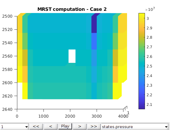
run two test cases
datadir = getDatasetPath('aquifertest', 'download', true);

for icase = 1 : 2
fnroot = sprintf('2D_OILWATER_AQ_ECLIPSE_%d', icase);
    fn = fullfile(datadir, [fnroot, '.DATA']);
    [model, initState, schedule] = setupAquifertest(fn);
    [wellSols, states, schedulereport] = simulateScheduleAD(initState, model, ...
                                                      schedule);
    statesEcl = loadAquiferEclipseResult(datadir, fnroot);
No converter needed in section 'REGIONS'.
No converter needed in section 'SUMMARY'.
Adding 40 artificial cells at top/bottom

Processing regular i-faces
 Found 144 new regular faces
Elapsed time is 0.018308 seconds.

...
No converter needed in section 'REGIONS'.
No converter needed in section 'SUMMARY'.
Adding 40 artificial cells at top/bottom

Processing regular i-faces
 Found 144 new regular faces
Elapsed time is 0.007527 seconds.

...
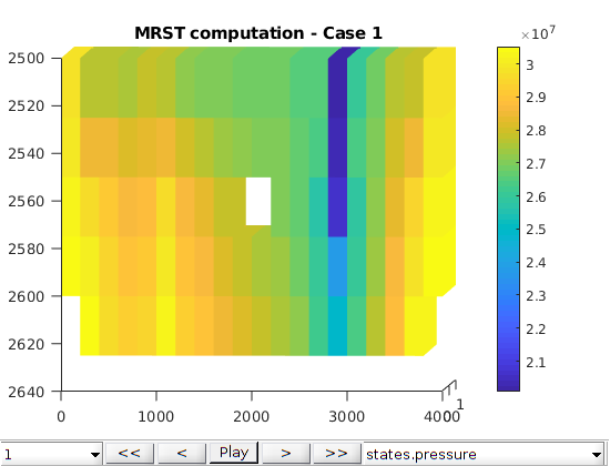
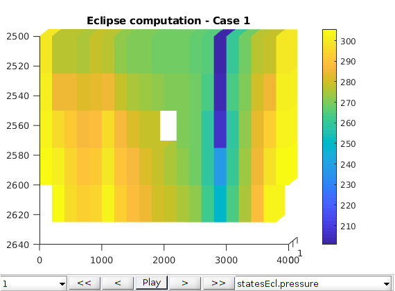
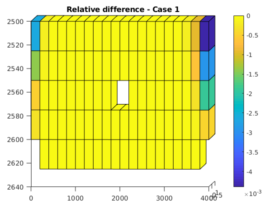
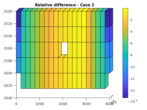
plots
G = model.G;
    figure
    plotToolbar(G, states);
    view([2, 2]);
    colorbar
    title(sprintf('MRST computation - Case %d', icase));
    figure
    plotToolbar(G, statesEcl);
    view([2, 2]);
    colorbar
    title(sprintf('Eclipse computation - Case %d', icase));

    p = states{end}.pressure;
    pecl = statesEcl{end}.pressure;
    pecl = pecl*barsa;
    err = (p - pecl)./pecl;
    figure
    plotCellData(G, err);
    view([2, 2]);
    colorbar
    title(sprintf('Relative difference - Case %d', icase));

nd

% <html>
% <p><font size="-1
Example demonstrating use of boundary conditions for pressure support
Generated from blackoilSectorModelExample.m
We take the SPE1 fluid model to get a simple blackoil-model. We make the aqueous phase mobile by manually setting the relative permeability.
mrstModule add ad-core ad-blackoil ad-props
[~, ~, fluid, deck] = setupSPE1();
fluid.krW = @(s) s.^2;
No converter needed in section 'REGIONS'.
No converter needed in section 'SUMMARY'.
Adding 200 artificial cells at top/bottom

Processing regular i-faces
 Found 550 new regular faces
Elapsed time is 0.001533 seconds.

...
Set up a simple grid with an initial state
We create a small grid with initial water and oil saturation, as well as a Rs (dissolved gas in oil-ratio) of 200. This undersaturated reservoir does not have any free gas.
G = cartGrid([50, 50, 1], [1000, 1000, 100]*meter);
G = computeGeometry(G);

rock = makeRock(G, 0.3*darcy, 0.3);

% Define initial composition and pressure
s0 = [0.2, 0.8, 0];
p0 = 300*barsa;
state0 = initResSol(G, p0, s0);
state0.rs = repmat(200, G.cells.num, 1);
% Black oil with disgas
model = ThreePhaseBlackOilModel(G, rock, fluid, 'disgas', true);
Processing Cells    1 : 2500 of 2500 ... done (0.02 [s], 1.16e+05 cells/second)
Total 3D Geometry Processing Time = 0.022 [s]
Set up driving forces
We will operate a single producer well at a fixed rate. In addition, we define a set of boundary conditions at the vertical boundary of the domain with a fixed pressure and composition equal to the initial values of the reservoir itself.
% Time horizon
T = 10*year;
% Produce 1/4 PV at surface conditions controlled by oil rate
ij = ceil(G.cartDims./2);
W = verticalWell([], G, rock, ij(1), ij(2), [], ...
    'val',      -0.25*sum(model.operators.pv)/T, ...
    'type',     'orat',...
    'comp_i',   [1, 1, 1]/3, ...
    'sign',     -1, ...
    'name',     'Producer');
% Define a lower bhp limit so that we have a lower bound on the reservoir
% pressure during the simulation.
W.lims.bhp = 100*barsa;

% Define boundary conditions
bc = [];
sides = {'xmin', 'xmax', 'ymin', 'ymax'};
for side = 1:numel(sides)
    bc = pside(bc, G, sides{side}, p0, 'sat', s0);
end
% We define initial Rs value for the BC. We can either supply a single
% value per interface or one for all interfaces. In this case, we supply a
% single value for all interfaces since there is no variation in the
% initial conditions.
%
% To define dissolution per face, a matrix of dimensions numel(bc.face)x3x3
% would have to be set.
bc.dissolution = [1, 0,   0;...
% Water fractions in phases
                  0, 1,   0; ...% Oil fractions in phases
                  0, 200, 1];   % Gas fractions in phases
% Simple uniform schedule with initial rampup
dt = rampupTimesteps(T, 30*day);

% Define schedule with well and constant pressure boundary conditions
schedule = simpleSchedule(dt, 'W', W, 'bc', bc);
[ws, states] = simulateScheduleAD(state0, model, schedule);

% Define schedule with well and closed boundaries
schedule2 = simpleSchedule(dt, 'W', W, 'bc', []);
[ws_c, states_c] = simulateScheduleAD(state0, model, schedule2);
Defaulting reference depth to top of formation for well Producer. Please specify 'refDepth' optional argument to 'addWell' if you require bhp at a specific depth.
*****************************************************************
********** Starting simulation:   130 steps,  3650 days *********
*****************************************************************
Preparing model for simulation...
Model ready for simulation...
Preparing schedule for simulation...
Schedule ready for simulation...
...
Compare the two results
We observe that the simulation with constant boundary pressure has a very different pressure build up than the same problem with closed boundaries. Note also that once the bhp limit is reached, the well switches controls in the closed model, and the oil production rate changes.
plotWellSols({ws, ws_c}, cumsum(schedule.step.val), ...
    'datasetnames', {'Constant pressure', 'Closed boundaries'})
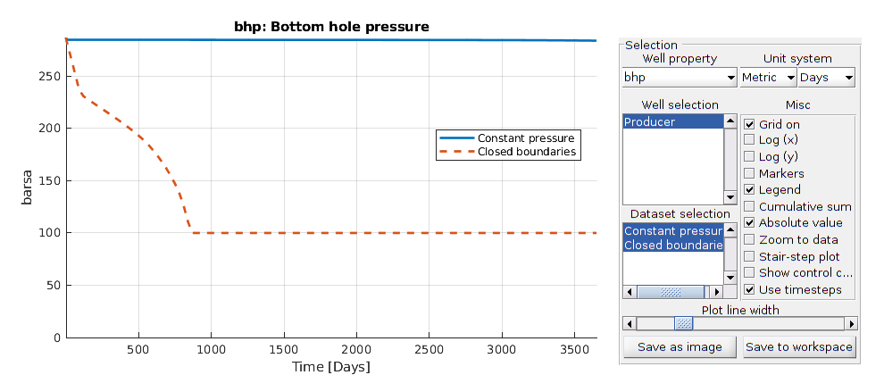
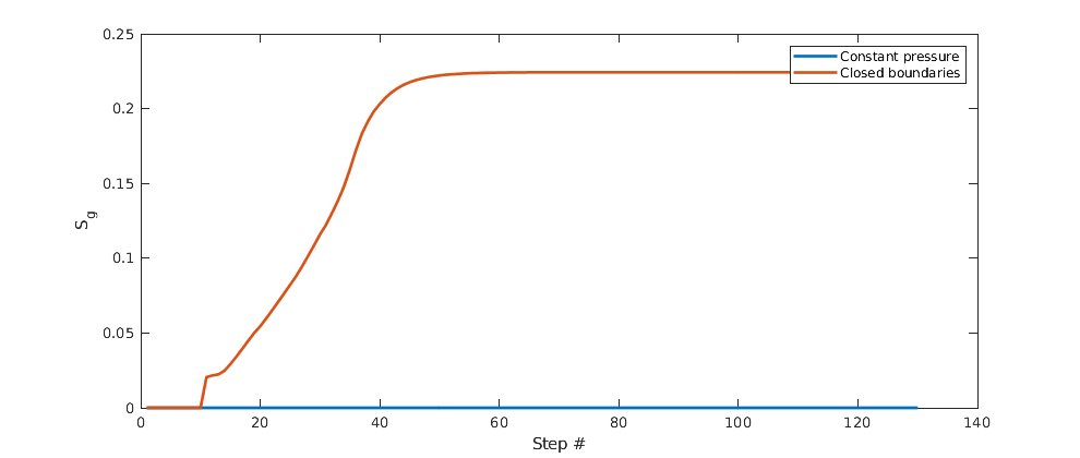
Plot the gas in the well cells
If we do not have open boundaries, the pressure will eventually drop as a result of the large removed volumes of oil and dissolved gas. For the model with closed boundaries, we get drop-out of free gas.
as_open = cellfun(@(x) x.s(W.cells(1), 3), states);
gas_closed = cellfun(@(x) x.s(W.cells(1), 3), states_c);

clf;
plot([gas_open, gas_closed], 'linewidth', 2)
ylabel('S_g')
xlabel('Step #');
legend('Constant pressure', 'Closed boundaries');

% <html>
% <p><font size="-1
mrstModule add ad-core ad-blackoil deckformat ad-props linearsolvers
mrstVerbose on
[G, rock, fluid, deck, state] = setupSPE1();
[state0, model, schedule] = initEclipseProblemAD(deck);
No converter needed in section 'REGIONS'.
No converter needed in section 'SUMMARY'.
Adding 200 artificial cells at top/bottom

Processing regular i-faces
 Found 550 new regular faces
Elapsed time is 0.006345 seconds.

...
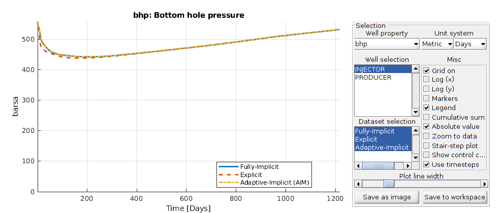
Fully-implicit
Generated from blackoilTimeIntegrationExample.m
The default discretization in MRST is fully-implicit. Consequently, we can use the model as-is.
implicit = packSimulationProblem(state0, model, schedule, 'SPE1_ex', 'Name', 'Fully-Implicit');
Explicit solver
This solver has a time-step restriction based on the CFL condition in each cell. The solver estimates the time-step before each solution.
model_explicit = model.validateModel();
% Get the flux discretization
flux = model_explicit.FluxDiscretization;
% Use explicit form of flow state
fb = ExplicitFlowStateBuilder();
flux = flux.setFlowStateBuilder(fb);
model_explicit.FluxDiscretization = flux;
explicit = packSimulationProblem(state0, model_explicit, schedule, 'SPE1_ex', 'Name', 'Explicit');
Adaptive implicit
We can solve some cells implicitly and some cells explicitly based on the local CFL conditions. For many cases, this amounts to an explicit treatment far away from wells or driving forces. The values for estimated composition CFL and saturation CFL to trigger a switch to implicit status can be adjusted.
model_aim = model.validateModel();
flux = model_aim.FluxDiscretization;
fb = AdaptiveImplicitFlowStateBuilder();
flux = flux.setFlowStateBuilder(fb);
model_aim.FluxDiscretization = flux;
aim = packSimulationProblem(state0, model_aim, schedule, 'SPE1_ex', 'Name', 'Adaptive-Implicit (AIM)');
Simulate the problems
problems = {implicit, explicit, aim};
simulatePackedProblem(problems);
*******************************************************
* Case "SPE1_ex" (Fully-Implicit)                     *
* Description: "Fully-Implicit_GenericBlackOilModel"  *
*******************************************************
-> Complete output found, nothing to do here.

*************************************************
* Case "SPE1_ex" (Explicit)                     *
...
Get output and plot the well results
There are oscillations in the well curves. Increasing the CFL limit beyond unity will eventually lead to oscillations.
[ws, states, reports, names, T] = getMultiplePackedSimulatorOutputs(problems);
plotWellSols(ws, T, 'datasetnames', names);
Found complete data for SPE1_ex (Fully-Implicit): 120 steps present
Found complete data for SPE1_ex (Explicit): 120 steps present
Found complete data for SPE1_ex (Adaptive-Implicit (AIM)): 120 steps present
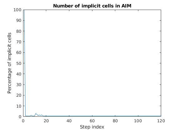
Plot the fraction of cells which are implicit
imp_frac = cellfun(@(x) sum(x.implicit)/numel(x.implicit), states{3});
figure;
plot(100*imp_frac);
title('Number of implicit cells in AIM')
ylabel('Percentage of implicit cells')
xlabel('Step index')
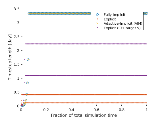
Plot the time-steps taken
The implicit solvers use the control steps while the explicit solver must solve many substeps.
igure; hold on
markers = {'o', '.', 'x'};
for i = 1:numel(reports)
    dt = getReportMinisteps(reports{i});
    x = (1:numel(dt))/numel(dt);
    plot(x, dt/day, 'marker', markers{i})
end
xlabel('Timestep length [day]')
legend(names)

% <html>
% <p><font size="-1
Gravity segregation using two phase AD solvers
Generated from blackoilTutorialGravSeg.m
This example demonstrates a simple, but classical test problem for a multiphase solver. The problem we are considering is that of gravity segregation: For a given domain, we let the initial fluid distribution consist of a dense fluid atop of a lighter one. Gravity is the only active force, and bouyancy will over time force the reservoir towards a stable equilibrium in which the denser fluid has switched place with the lighter fluid. The example also demonstrates how to set up a simple schedule (one or more timesteps with a collection of driving forces such as bc and wells).
mrstModule add ad-core ad-blackoil ad-props mrst-gui
Reservoir geometry and petrophysical properties
We begin by defining a simple homogenous reservoir of 1 by 1 by 5 meters and 250 simulation cells.
dims = [5 5 10];
G = cartGrid(dims, [1, 1, 5]*meter);
G = computeGeometry(G);

rock = makeRock(G, 100*milli*darcy, 0.5);
Processing Cells   1 : 250 of 250 ... done (0.00 [s], 6.98e+04 cells/second)
Total 3D Geometry Processing Time = 0.004 [s]
Defining the fluid properties
In this section, we set up a generic fluid suitable for solvers based on automatic differentiation. The fluid model is by default incompressible. We define two phases: Oil and water with significant differences in density and viscosity.
fluid = initSimpleADIFluid('phases', 'WO', ...
                           'mu', [1, 10]*centi*poise, ...
                           'n',  [1, 1], ...
                           'rho', [1000, 700]*kilogram/meter^3);
Defining the model
The model object contains all functions necessary to simulate a mathematical model using the AD-solvers. In our case, we are interested in a standard fully implicit two-phase oil/water model. By passing the grid, rock, and fluid into the model constructor we obtain a model with precomputed operators and quantities that can be passed on to the simulator. We also ensure that gravity is enabled before we call the constructor.
gravity reset on
model = TwoPhaseOilWaterModel(G, rock, fluid);

% Show the model
disp(model)
TwoPhaseOilWaterModel with properties:

                   disgas: 0
                   vapoil: 0
                drsMaxRel: Inf
                drsMaxAbs: Inf
                    fluid: [1×1 struct]
                     rock: [1×1 struct]
...
Set up initial state
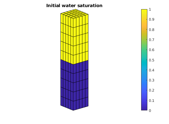
We must also define the initial state. The state contains the unstable initial fluid distribution. We do this by setting the water saturation to 1 in all cells and then setting it to zero in cells below a datum point. We defined the water (first phase) density to be 1000 kg/m^3 when we set up the fluid model. Note that we let the pressure be uniform initially. The model is relatively simple, so we do not need to worry about the initial pressure being reasonable, but this is something that should be considered more carefullly for models with e.g., compressibility. To ensure that we got the distribution right, we make a plot of the initial saturation.
[ii, jj, kk] = gridLogicalIndices(G);

lower = kk > 5;
sW = ones(G.cells.num, 1);
sW(lower) = 0;
s = [sW, 1 - sW];

% Finally set up the state
state = initResSol(G, 100*barsa, s);

% Plot the initial water saturation
figure;
plotCellData(G, state.s(:, 1))
axis equal tight off
view(50, 20)
title('Initial water saturation')
colorbar, drawnow
Set up boundary conditions and timesteps
Finally, we add a simple boundary condition of 100 bar pressure at the bottom of the reservoir. This is not strictly required, but the incompressible model will produce singular linear systems if we do not fix the pressure somehow. It is well known that the pressure is not unique for an incompressible model if there are no Dirichlet boundary conditions, as multiple pressures will give the same velocity field. Another alternative would be to add (some) compressibility to our fluid model. Once we have set up the boundary conditions, we define 20 timesteps of 90 days each, which is enough for the state to approach equilibrium. The simulator will cut timesteps if they do not converge, so we are not overly worried about the large initial timestep when the problem is the most stiff. Finally, we combine the timesteps and the boundary conditions into a schedule. A schedule collects multiple timesteps into a single struct and makes it easier to have for example different boundary conditions at different time periods. For this example, however, the schedule is very simple.
bc = [];
bc = pside(bc, G, 'ZMin', 100*barsa, 'sat', [0 1]);

dt = repmat(90*day, 20, 1);

schedule = simpleSchedule(dt, 'bc', bc);
Simulate the problem
Finally, we simulate the problem. We note that the three simple objects define the entire simulation: - state defines the initial values in the reservoir - model defines the partial differential equations, their physical constraints and the numerical discretizations required to advance from one time to the next. - schedule defines any time dependent input parameters as well as the timesteps.
[wellSols, states] = simulateScheduleAD(state, model, schedule, 'Verbose', true);
*****************************************************************
********** Starting simulation:    20 steps,  1800 days *********
*****************************************************************
Preparing model for simulation...
Model ready for simulation...
Preparing schedule for simulation...
Schedule ready for simulation...
Validating initial state...
...
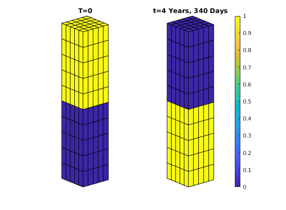
Plot the segregation process
We finish by plotting the water saturation at each timestep, showing how the lighter fluid migrates upward and the heavier fluid downward.
colorbar off; title('T=0');
set(gca,'Position',[.13 .11 .335 .815]); subplot(1,2,2);
for i = 1:numel(states)
    %figure(h); clf;

    % Neat title
    str = ['t=', formatTimeRange(sum(dt(1:i)))];

    % Plotting
    plotCellData(G, states{i}.s(:, 1))
    title(str)

    % Make axis equal to show column structure
    axis equal tight off
    view(50, 20)
    colorbar
    caxis([0, 1])

    drawnow, pause(0.2)
end
Copyright notice
<html>
% <p><font size="-1
Example demonstrating accelerated assembly for faster simulation
Generated from blackoilTutorialMexAcceleration.m
Running larger cases in MRST is possible, but the default parameters of MRST’s solvers are optimized for ease-of-use out of the box with just a standard Matlab installation. We do not wish to require users to have C++ compilers, external software or expensive add-on toolboxes to make use of the software. However, simulation can be achieved much faster if one has access to both - A C++ compiler - An external linear solver with a Matlab interface. This examples demonstrates the use of MEX to seamlessly improve assembly speed for AD-solvers.
mrstModule add ad-core ad-blackoil deckformat ad-props linearsolvers
Define a 70x70x30 grid with uniform properties
Obviously, you can adjust this to test your setup
dims = [70, 70, 30];
pdims = [1000, 1000, 100]*meter;
G = cartGrid(dims, pdims);
G = computeGeometry(G);
rock = makeRock(G, 0.1*darcy, 0.3);
Processing Cells      1 :  18375 of 147000 ... done (0.16 [s], 1.14e+05 cells/second)
Processing Cells  18376 :  36750 of 147000 ... done (0.14 [s], 1.33e+05 cells/second)
Processing Cells  36751 :  55125 of 147000 ... done (0.14 [s], 1.34e+05 cells/second)
Processing Cells  55126 :  73500 of 147000 ... done (0.14 [s], 1.33e+05 cells/second)
Processing Cells  73501 :  91875 of 147000 ... done (0.14 [s], 1.33e+05 cells/second)
Processing Cells  91876 : 110250 of 147000 ... done (0.14 [s], 1.32e+05 cells/second)
Processing Cells 110251 : 128625 of 147000 ... done (0.14 [s], 1.34e+05 cells/second)
Processing Cells 128626 : 147000 of 147000 ... done (0.14 [s], 1.34e+05 cells/second)
...
Set up QFS water injection scenario
As the point of this example is on how to set up the solvers, we just set up a simple injection scenario for a 3D quarter-five-spot problem.
gravity reset on
time = 10*year;
irate = 0.3*sum(poreVolume(G, rock)/time);

W = [];
W = verticalWell(W, G, rock, 1, 1, [], 'comp_i', [1, 0, 0], ...
                'type', 'rate', 'val', irate);
W = verticalWell(W, G, rock, dims(1), dims(2), 1, 'comp_i', [1, 0, 0], ...
                 'type', 'bhp', 'val', 100*barsa);
Defaulting reference depth to top of formation for well W1. Please specify 'refDepth' optional argument to 'addWell' if you require bhp at a specific depth.
Defaulting reference depth to top of formation for well W2. Please specify 'refDepth' optional argument to 'addWell' if you require bhp at a specific depth.
Three-phase fluid model with compressibility and nonlinear flux
fluid = initSimpleADIFluid('n', [2, 3, 1], ...
                           'rho', [1000, 700, 10], ...
                           'mu', [1, 5, 0.1]*centi*poise, ...
                           'c', [0, 1e-6, 1e-4]/barsa);
Do 5 time-steps of 30 days each to test assembly speed
dt = repmat(30*day, 5, 1);
% Alternatively: Run the whole schedule with 200 time-steps.
% dt = rampupTimesteps(time, time/200);
schedule = simpleSchedule(dt, 'W', W);

model = GenericBlackOilModel(G, rock, fluid, 'disgas', false, 'vapoil', false);
Set up mex-accelerated backend and reduced variable set for wells
We use the Diagonal autodiff backend to calculate derivatives. By default, this uses only Matlab, so we also set the “useMex” flag to be true. It will then use C++ versions of most discrete operators during assembly.
model.AutoDiffBackend = DiagonalAutoDiffBackend('useMex', true);
model = model.validateModel();
model.FacilityModel.primaryVariableSet = 'bhp';
Run assembly tests (will compile backends if required)
Note: Benchmarks are obviously not accurate if compilation is performed.
testMexDiagonalOperators(model, 'block_size', 3);
********************************************************
* Face average
* Diagonal: 0.024513s, Diagonal-MEX: 0.013615s (1.80 speedup)
*   Sparse: 0.018307s, Diagonal-MEX: 0.013615s (1.34 speedup)
Value error 0, Jacobian error 0
********************************************************
********************************************************
* Single-point upwind
...
Set up a compiled linear solver
We use a AMGCL-based CPR solver to solve the problem. It is sufficient to have a working C++ compiler, the AMGCL repository and BOOST available to compile it. See the documentation of amgcl_matlab for more details on how to set up these paths.
ncomp = model.getNumberOfComponents();
solver = AMGCL_CPRSolverAD('tolerance', 1e-3, 'block_size', ncomp, ...
                            'useSYMRCMOrdering', true, ...
                            'coarsening', 'aggregation', 'relaxation', 'ilu0');

nls = NonLinearSolver('LinearSolver', solver);
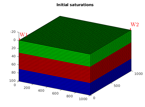
Set up initial state
We define fluid contacts and datum pressure
region = getInitializationRegionsBlackOil(model, [70, 30], 'datum_pressure', 200*barsa);
state0 = initStateBlackOilAD(model, region);

figure(1); clf
plotCellData(G, state0.s(:, [2, 3, 1]));
view(30, 30);
plotWell(G, W);
title('Initial saturations');
Run a serial simulation
maxNumCompThreads(1)
[ws0, states0, rep0] = simulateScheduleAD(state0, model, schedule, 'NonLinearSolver', nls);
ans =

     8

*****************************************************************
********** Starting simulation:     5 steps,   150 days *********
*****************************************************************
...
Run a parallel simulation with four threads
maxNumCompThreads(4)
[ws, states, rep] = simulateScheduleAD(state0, model, schedule, 'NonLinearSolver', nls);
% Reset max number of threads
N = maxNumCompThreads('automatic');
ans =

     1

*****************************************************************
********** Starting simulation:     5 steps,   150 days *********
*****************************************************************
...
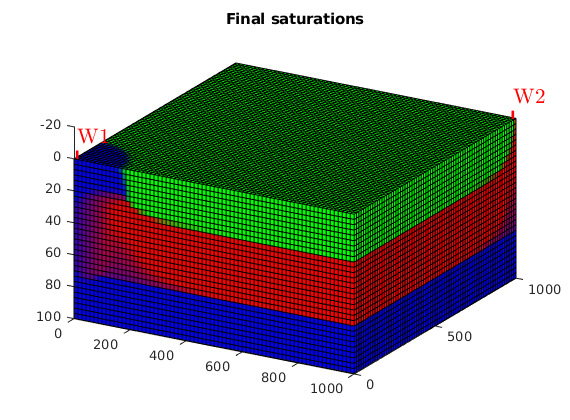
Plot the final saturations
figure(1); clf
plotCellData(G, states{end}.s(:, [2, 3, 1]));
view(30, 30);
plotWell(G, W);
title('Final saturations');
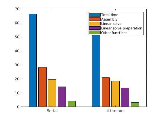
Plot timings
We plot the total time, the assembly (linearization) time, the linear solver time and the linear solver preparation time. The assembly and linear solver time are in general parallel, while the preparation is currently not. We likely observe that the linear solver is the place where most of the time is spent: Manipulating sparse matrices to fit them to an external solver can take significant time for a moderate-size problem.
serial = getReportTimings(rep0);
par = getReportTimings(rep);

total0 = sum(vertcat(serial.Total));
assembly0 = sum(vertcat(serial.Assembly));
lsolve0 = sum(vertcat(serial.LinearSolve));
lsolve_prep0 = sum(vertcat(serial.LinearSolvePrep));
its0 = rep0.Iterations;

total = sum(vertcat(par.Total));
assembly = sum(vertcat(par.Assembly));
lsolve = sum(vertcat(par.LinearSolve));
lsolve_prep = sum(vertcat(par.LinearSolvePrep));
its = rep.Iterations;

a = [total0, assembly0, lsolve0, lsolve_prep0];
b = [total, assembly, lsolve, lsolve_prep];

a(end+1) = a(1) - sum(a(2:end));
b(end+1) = b(1) - sum(b(2:end));

figure;
bar([a; b])
legend('Total time', 'Assembly', 'Linear solve', 'Linear solve preparation', 'Other functions')
set(gca, 'XTickLabel', {'Serial', [num2str(N), ' threads']})
Other notes
We note that the more degrees-of-freedom you have per cell in your model, the more efficient the MEX operators are compared to Matlab. See e.g. the compositional module’s example “compositionalLargerProblemTutorial.m” for another example benchmark.
<html>
% <p><font size="-1
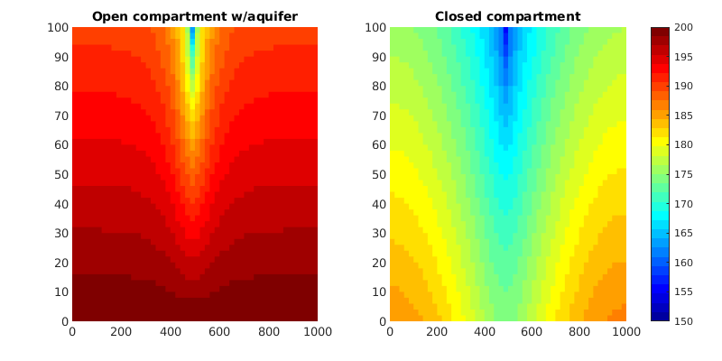
Example: Depletion of a closed or open reservoir compartment
Generated from blackoilTutorialOnePhase.m
In this tutorial, we will show how to set up a simulator from scratch in the automatic differentiation, object-oriented (AD-OO) framework without the use of input files. As an example we consider a 2D rectangular reservoir compartment with homogeneous properties, drained by a single producer at the midpoint of the top edge. The compartment is either closed (i.e., sealed by no-flow boundary conditions along all edges), or open with constant pressure support from an underlying, infinite aquifer, which we model as a constant-pressure boundary condition.
mrstModule add ad-props ad-core ad-blackoil
Grid, petrophysics, and fluid objects
To create a complete model object using the AD-OO framework, we first need to define three standard MRST structures representing the grid and the rock and fluid properties
% The grid and rock model
G    = computeGeometry(cartGrid([50 50],[1000 100]));
rock = makeRock(G, 100*milli*darcy, 0.3);

% Fluid properties
pR  = 200*barsa;
fluid = initSimpleADIFluid('phases','W',           ...
% Fluid phase: water
                           'mu',  1*centi*poise,   ...
% Viscosity
                           'rho', 1000,            ...
% Surface density [kg/m^3]
                           'c',   1e-4/barsa,      ...
% Fluid compressibility
                           'cR',  1e-5/barsa       ...
% Rock compressibility
                           );
Computing normals, areas, and centroids...    Elapsed time is 0.002116 seconds.
Computing cell volumes and centroids...               Elapsed time is 0.007661 seconds.
Make Reservoir Model
We can now use the three objects defined above to instantiate the reservoir model. To this end, we will use a WaterModel, which is a specialization of the general ReservoirModel implemented in ad-core. The only extra thing we need to do is to explicitly set the gravity direction. By default, the gravity in MRST is a 3-component vector that points in the positive z-direction. Here, we set it to a 2-component vector pointing in the negative y-direction.
gravity reset on
wModel = WaterModel(G, rock, fluid,'gravity',[0 -norm(gravity)]);
% Prepare the model for simulation.
wModel = wModel.validateModel();
Drive mechansims and schedule
The second thing we need to specify is the mechanisms that will drive flow in the reservoir, i.e., the wells and boundary conditions. These may change over time and MRST therefore uses the concept of a schedule that describes how the drive mechansims change over time. In our case, we use the same setup for the whole simulation. The schedule also enables us to specify the time steps we wish the simulator to use, provided that these give convergent and stable computations. (If not, the simulator may cut the time step).
% Well: at the midpoint of the south edge
wc = sub2ind(G.cartDims, floor(G.cartDims(1)/2), G.cartDims(2));
W = addWell([], G, rock,  wc,     ...
        'Type', 'bhp', 'Val', pR-50*barsa, ...
        'Radius', 0.1, 'Name', 'P1','Comp_i',1,'sign',1);

% Boundary conditions: fixed pressure at bottom and no-flow elsewhere
bc=pside([],G,'South',200*barsa,'sat',1);

% Schedule: describing time intervals and corresponding drive mechanisms
schedule1 = simpleSchedule(diff(linspace(0,5*day,41)), 'bc', bc, 'W', W);
schedule2 = simpleSchedule(diff(linspace(0,5*day,41)), 'W', W);
Defaulting reference depth to top of formation for well P1. Please specify 'refDepth' optional argument to 'addWell' if you require bhp at a specific depth.
Reservoir state
The last component we need in order to specify our reservoir model is the reservoir state, i.e., the fluid pressure. For multiphase models, the state also includes the phase saturations and compositions. In our case, we first set a constant pressure, and call on a solver from ad-core to compute vertical equilibrium.
state = initResSol(G, pR); % Constant pressure
state.wellSol = initWellSolAD([], wModel, state); % No well initially
% Vertical equilibrium
verbose = false;
nonlinear = NonLinearSolver();
state = nonlinear.solveTimestep(state, 10000*day, wModel, 'bc', bc);
clf,
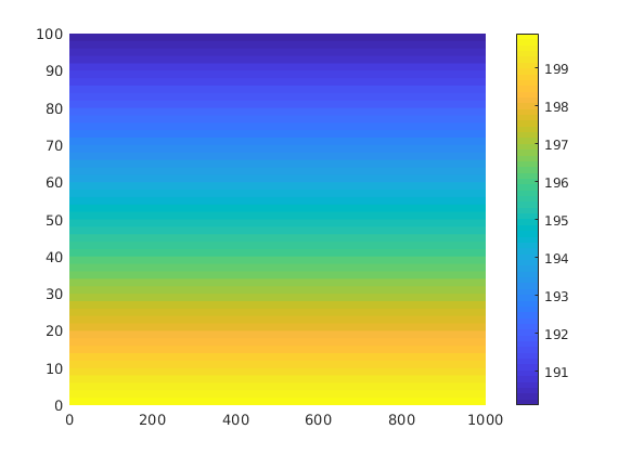
plotCellData(G,state.pressure/barsa,'EdgeColor','none');
colorbar
=======================
| It # | water (cell) |
=======================
|    1 | 2.01e-05     |
|    2 |*1.99e-08     |
=======================
Solved timestep with 1 accepted ministep (0 rejected, 1 total iteration)
Run simulations
To make the case a bit more interesting, we compute the flow problem twice. The first simulation uses the prescribed boundary conditions, which will enable fluids to pass out of the north boundary. In the second simulation, we close the system by imposing no-flow conditions also on the north boundary
% Simulation pressure 200 bar at top
[wellSols1, states1] = simulateScheduleAD(state, wModel, schedule1);

% Simulation with no-flow at top
[wellSols2, states2] = simulateScheduleAD(state, wModel, schedule2);
*****************************************************************
********** Starting simulation:    40 steps,     5 days *********
*****************************************************************
Preparing model for simulation...
Model ready for simulation...
Preparing schedule for simulation...
Schedule ready for simulation...
Validating initial state...
...
Plot results
Prepare animation
wpos = G.cells.centroids(wc,:); clf
set(gcf,'Position',[600 400 800 400])
h1 = subplot('Position',[.1 .11 .34 .815]);
hp1 = plotCellData(G,state.pressure/barsa,'EdgeColor','none');
title('Open compartment w/aquifer'); caxis([pR/barsa-50 pR/barsa]);
h2 = subplot('Position',[.54 .11 .4213 .815]);
hp2 = plotCellData(G,state.pressure/barsa,'EdgeColor','none');
title('Closed compartment'); caxis([pR/barsa-50 pR/barsa]);
colormap(jet(32)); colorbar
% Animate solutions by resetting CData property of graphics handle
for i=1:numel(states1)
set(hp1,'CData', states1{i}.pressure/barsa);
set(hp2,'CData', states2{i}.pressure/barsa);
drawnow, pause(0.1);
end
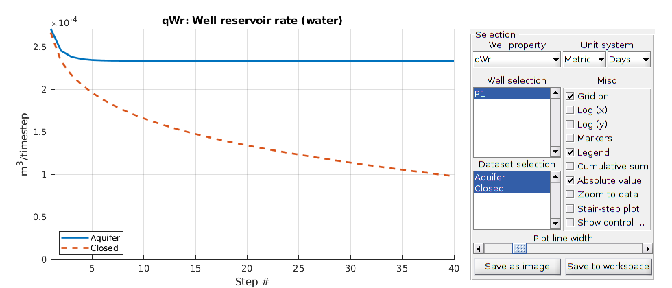
% Launch plotting of well responses
plotWellSols({wellSols1,wellSols2}, ...
'Datasetnames',{'Aquifer','Closed'}, 'field','qWr');
Copyright notice
<html>
% <p><font size="-1
Example demonstrating in-situ plotting capabilities in MRST-AD
Generated from blackoilTutorialPlotHook.m
The AD-solvers allow for dynamic plotting during the simulation process. This example demonstrates this capability using “plotWellSols” and a panel showing simulation progress. We first set up a simulation model of SPE1 in the standard manner.
mrstModule add ad-core ad-blackoil ad-props mrst-gui deckformat

[G, rock, fluid, deck, state0] = setupSPE1();
model = selectModelFromDeck(G, rock, fluid, deck);
schedule = convertDeckScheduleToMRST(model, deck);
No converter needed in section 'REGIONS'.
No converter needed in section 'SUMMARY'.
Adding 200 artificial cells at top/bottom

Processing regular i-faces
 Found 550 new regular faces
Elapsed time is 0.010813 seconds.

...
Set up plotting function
We set up a function handle that takes in the current simulator variables, which will be run after each succesful control step. This function can also pause the simulation or change the maximum timestep as a proof of concept.
close all
fn = getPlotAfterStep(state0, model, schedule, 'plotWell', true,...
                                               'plotReservoir', false);
disp(fn)
@(model,states,reports,solver,schedule,simtime)afterStepFunction(model,states,reports,solver,schedule,simtime,injData,injectWell,hdata,hwell)
Run the simulation with plotting function
linsolve = selectLinearSolverAD(model);
[wellSols, states, report] = simulateScheduleAD(state0, model, schedule, ...
    'Verbose', true, 'afterStepFn', fn, 'linearsolver', linsolve);
*****************************************************************
********** Starting simulation:   120 steps,  1216 days *********
*****************************************************************
Preparing model for simulation...
Model ready for simulation...
Preparing schedule for simulation...
Schedule ready for simulation...
Validating initial state...
...
Copyright notice
<html>
% <p><font size="-1
mrstModule add ad-core ad-blackoil deckformat ad-props linearsolvers
mrstVerbose on
L = 1000*meter;
G = cartGrid(150, L);
G = computeGeometry(G);

x = G.cells.centroids/L;

poro = repmat(0.5, G.cells.num, 1);
poro(x > 0.2 & x < 0.3) = 0.05;
poro(x > 0.7 & x < 0.8) = 0.05;
poro(x > 0.45 & x < 0.55) = 0.1;

rock = makeRock(G, 1*darcy, poro);

close all
plot(poro)
time = 500*day;

% Default oil-water fluid with unit values
fluid = initSimpleADIFluid('phases', 'WO', 'n', [1 1]);

% Set up model and initial state.
model = GenericBlackOilModel(G, rock, fluid, 'gas', false);
state0 = initResSol(G, 50*barsa, [0, 1]);

% Set up drive mechanism: constant rate at x=0, constant pressure at x=L
pv = poreVolume(G, rock);
injRate = sum(pv)/time;
bc = fluxside([], G, 'xmin', injRate, 'sat', [1, 0]);
bc = pside(bc, G, 'xmax', 0*barsa, 'sat', [0, 1]);

n  = 150;
dT = time/n;
timesteps = rampupTimesteps(time, dT, 8);
schedule = simpleSchedule(timesteps, 'bc', bc);
Fully-implicit
Generated from immiscibleTimeIntegrationExample.m
The default discretization in MRST is fully-implicit. Consequently, we can use the model as-is.
implicit = packSimulationProblem(state0, model, schedule, 'immiscible_time', 'Name', 'Fully-Implicit');
Explicit solver
This solver has a time-step restriction based on the CFL condition in each cell. The solver estimates the time-step before each solution.
model_explicit = model.validateModel();
% Get the flux discretization
flux = model_explicit.FluxDiscretization;
% Use explicit form of flow state
fb = ExplicitFlowStateBuilder('Verbose', true);
fb.compositionCFL = inf;
flux = flux.setFlowStateBuilder(fb);
model_explicit.FluxDiscretization = flux;
explicit = packSimulationProblem(state0, model_explicit, schedule, 'immiscible_time', 'Name', 'Explicit');
Adaptive implicit
We can solve some cells implicitly and some cells explicitly based on the local CFL conditions. For many cases, this amounts to an explicit treatment far away from wells or driving forces. The values for estimated composition CFL and saturation CFL to trigger a switch to implicit status can be adjusted.
model_aim = model.validateModel();
flux = model_aim.FluxDiscretization;
fb = AdaptiveImplicitFlowStateBuilder('Verbose', true);
fb.compositionCFL = inf;
flux = flux.setFlowStateBuilder(fb);
model_aim.FluxDiscretization = flux;
aim = packSimulationProblem(state0, model_aim, schedule, 'immiscible_time', 'Name', 'Adaptive-Implicit (AIM)');
Make an explicit solver with larger CFL limit
Since the equation is linear, we can set the NonLinearSolver to use a single step. We bypass the convergence checks and can demonstrate the oscillations that result in taking a longer time-step than the stable limit.
model_explicit_largedt = model.validateModel();
% Get the flux discretization
flux = model_explicit_largedt.FluxDiscretization;
% Use explicit form of flow state
fb = ExplicitFlowStateBuilder();
fb.saturationCFL = 5;
fb.compositionCFL = inf; % Immiscible, saturation cfl is enough
flux = flux.setFlowStateBuilder(fb);
model_explicit_largedt.FluxDiscretization = flux;
model_explicit_largedt.stepFunctionIsLinear = true;
explicit_largedt = packSimulationProblem(state0, model_explicit_largedt, schedule, 'immiscible_time', 'Name', 'Explicit (CFL target 5)');
Simulate the problems
problems = {implicit, explicit, aim, explicit_largedt};
simulatePackedProblem(problems, 'continueOnError', false);
*******************************************************
* Case "immiscible_time" (Fully-Implicit)             *
* Description: "Fully-Implicit_GenericBlackOilModel"  *
*******************************************************
-> Complete output found, nothing to do here.

*************************************************
* Case "immiscible_time" (Explicit)             *
...
Get output and plot the well results
There are oscillations in the well curves. Increasing the CFL limit beyond unity will eventually lead to oscillations.
[ws, states, reports, names, T] = getMultiplePackedSimulatorOutputs(problems);
Found complete data for immiscible_time (Fully-Implicit): 158 steps present
Found complete data for immiscible_time (Explicit): 158 steps present
Found complete data for immiscible_time (Adaptive-Implicit (AIM)): 158 steps present
Found complete data for immiscible_time (Explicit (CFL target 5)): 158 steps present
Plot the results
Note oscillations for CFL > 1.
figure(1);
for stepNo = 1:numel(schedule.step.val)
    clf;
    subplot(2, 1, 1);
    hold on
    for j = 1:numel(states)
        plotCellData(G, states{j}{stepNo}.s(:, 1))
    end
    legend(names);

    subplot(2, 1, 2); hold on;
    plotCellData(G, rock.poro);
    dt = schedule.step.val(stepNo);
    state = states{1}{stepNo};
    cfl = estimateSaturationCFL(model, state, dt);
    plotCellData(G, cfl);
    plotCellData(G, ones(G.cells.num, 1), 'Color', 'k');
    legend('Porosity', 'CFL', 'CFL stable limit');
    drawnow
end
Plot the fraction of cells which are implicit
imp_frac = cellfun(@(x) sum(x.implicit)/numel(x.implicit), states{3});
figure;
plot(100*imp_frac);
title('Number of implicit cells in AIM')
ylabel('Percentage of implicit cells')
xlabel('Step index')
Plot the time-steps taken
The implicit solvers use the control steps while the explicit solver must solve many substeps.
igure; hold on
markers = {'o', '.', 'x', '.'};
for stepNo = 1:numel(reports)
    dt = getReportMinisteps(reports{stepNo});
    x = (1:numel(dt))/numel(dt);
    plot(x, dt/day, markers{stepNo})
end
ylabel('Timestep length [day]')
xlabel('Fraction of total simulation time');
legend(names)

% <html>
% <p><font size="-1
Multi-segment well example based on SPE 1 benchmark model
Generated from multisegmentWellExample.m
This example demonstrates the use of multisegment wells in MRST. The default wells in MRST assume flow in the well happens on a very short time-scale compared to the reservoir and can thus be accurately modelled by an instantaneous model. For some problems, however, more sophisticated well models may be required. The multisegment well class in MRST supports transient flow in the well. In addition, the class also allows for a more fine-grained representation of the well itself where the effect of valves and friction models can be included per segment.
% Load necessary modules
mrstModule add ad-blackoil ad-props deckformat ad-core mrst-gui
Set up model based on SPE 1
We use the SPE 1 example to get a simple black-oil case to modify. For more details on this model, see the the example blackoilTutorialSPE1.m.
[G, rock, fluid, deck, state] = setupSPE1();
[nx, ny] = deal(G.cartDims(1),G.cartDims(2));

model = ThreePhaseBlackOilModel(G, rock, fluid, 'inputdata', deck);
% Add extra output
model.extraStateOutput = true;

% Convert the deck schedule into a MRST schedule
schedule = convertDeckScheduleToMRST(model, deck);
No converter needed in section 'REGIONS'.
No converter needed in section 'SUMMARY'.
Adding 200 artificial cells at top/bottom

Processing regular i-faces
 Found 550 new regular faces
Elapsed time is 0.008292 seconds.

...
Construct multisegment well, and replace producer in original example
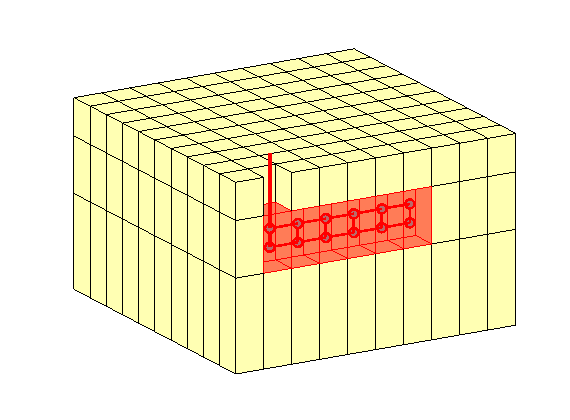
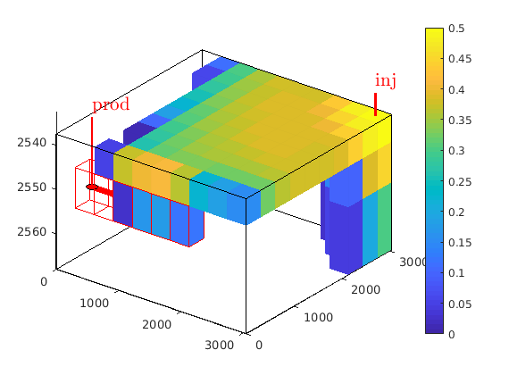
The well has 13 nodes. Nodes correspond to volumes in the well and are analogous to the grid cells used when the reservoir itself is discretized. The well is perforated in six grid blocks and we add nodes both for the wellbore and the reservoir contacts. By modelling the nodes in the reservoir contacts and the wellbore separately, we can introduce a valve between the reservoir and the wellbore. Nodes 1-7 represents the wellbore (frictional pressure drop) Well segments 2-8, 3-9, …, 7-13 will represent valves Only nodes 8-13 are connected to reservoir (grid-cells c1-c6)
% connection grid cells (along edge of second layer)
c = nx*ny + (2:7)';

% Make a conceptual illustration of the multisegment horizontal well
clf
flag=true(G.cells.num,1); flag([2; c])=false;
plotGrid(G,flag,'FaceColor',[1 1 .7]);
plotGrid(G,c,'FaceColor','r','FaceAlpha',.3,'EdgeColor','r','LineWidth',1);
x = G.cells.centroids(c,[1 1 1]); x(:,2) = NaN;
y = G.cells.centroids(c,[2 2 2]); y(:,2) = NaN;
z = G.cells.centroids(c,[3 3 3]); z(:,2) = NaN;
z(:,1) = z(:,1)+1.5; z(:,3) = z(:,3)-1.5;
hold on
plot3(x(1,[1 1]), y(1,[1 1]), z(1,1) - [0 15], '-r', 'LineWidth',3);
plot3(x, y, z,'-or','MarkerSize',7,'MarkerFaceColor',[.6 .6 .6],'LineWidth',2);
plot3(x(:,[1 3 2])',y(:,[1 3 2])',z(:,[1 3 2])','-r','LineWidth',2);
hold off, view(-30,25), axis tight off
First, initialize production well as “standard” well structure
prodS = addWell([], G, rock, c, 'name', 'prod', ...
                'refDepth', G.cells.centroids(1,3), ...
               'type', 'rate', 'val', -8e5*meter^3/day);

% Define additional properties needed for ms-well
% We have 12 node-to-node segments
topo = [1 2 3 4 5 6 2 3  4  5  6  7
        2 3 4 5 6 7 8 9 10 11 12 13]';
%      |   tubing  |    valves     |
% Create sparse cell-to-node mapping
cell2node = sparse((8:13)', (1:6)', 1, 13, 6);
% Segment lengths/diameters and node depths/volumes
lengths = [300*ones(6,1); nan(6,1)];
diam    = [.1*ones(6,1); nan(6,1)];
depths  = G.cells.centroids(c([1 1:end 1:end]), 3);
vols    = ones(13,1);
% Convert to ms-well
prodMS = convert2MSWell(prodS, 'cell2node', cell2node, 'topo', topo, 'G', G, 'vol', vols, ...
                   'nodeDepth', depths, 'segLength', lengths, 'segDiam', diam);

% Finally, we set flow model for each segment:
%   segments  1-6: wellbore friction model
%   segments 7-12: nozzle valve model
% The valves have 30 openings per connection
[wbix, vix]  = deal(1:6, 7:12);
[roughness, nozzleD, discharge, nValves] = deal(1e-4, .0025, .7, 30);

% Set up flow model as a function of velocity, density and viscosity
prodMS.segments.flowModel = @(v, rho, mu)...
    [wellBoreFriction(v(wbix), rho(wbix), mu(wbix), prodMS.segments.diam(wbix), ...
                      prodMS.segments.length(wbix), roughness, 'massRate'); ...
     nozzleValve(v(vix)/nValves, rho(vix), nozzleD, discharge, 'massRate')];

% In addition, we define a standard gas injector. Different well types can
% easily be combined in MRST, each with their own models for pressure drop
% and solution variables.
inj = addWell([], G, rock, 100, 'name', 'inj', 'type', 'rate', 'Comp_i', [0 0 1], ...
              'val', 2.5e6*meter^3/day,'refDepth', G.cells.centroids(1,3));
Run schedule with simple wells
We first simulate a baseline where the producer is treated as a simple well with instantaneous flow and one node per well-reservoir contact.
W_simple = [inj; prodS];
schedule.control.W = W_simple;

[wellSolsSimple, statesSimple] = simulateScheduleAD(state, model, schedule);
*****************************************************************
********** Starting simulation:   120 steps,  1216 days *********
*****************************************************************
Preparing model for simulation...
Model ready for simulation...
Preparing schedule for simulation...
Schedule ready for simulation...
Validating initial state...
...
Set up well models
We combine the simple and multisegment well together
W = combineMSwithRegularWells(inj, prodMS);
schedule.control.W = W;
% Initialize the facility model. This is normally done automatically by the
% simulator, but we do it explicitly on the outside to view the output
% classes. This approach is practical if per-well adjustments to e.g.
% tolerances are desired.

% First, validate the model to set up a FacilityModel
model = model.validateModel();
% Then apply the new wells to the FacilityModel
model.FacilityModel = model.FacilityModel.setupWells(W);

% View the simple injector
disp(model.FacilityModel.WellModels{1})
% View the multisegment producer
disp(model.FacilityModel.WellModels{2})
SimpleWell with properties:

                        W: [1×1 struct]
           allowCrossflow: 1
          allowSignChange: 0
    allowControlSwitching: 1
                 dpMaxRel: Inf
                 dpMaxAbs: Inf
...
Run the same simulation with multisegment wells
Note that if verbose output is enabled, the convergence reports will include additional fields corresponding to the well itself.
[wellSols, states, report] = simulateScheduleAD(state, model, schedule);
*****************************************************************
********** Starting simulation:   120 steps,  1216 days *********
*****************************************************************
Preparing model for simulation...
Model ready for simulation...
Preparing schedule for simulation...
Schedule ready for simulation...
Validating initial state...
...
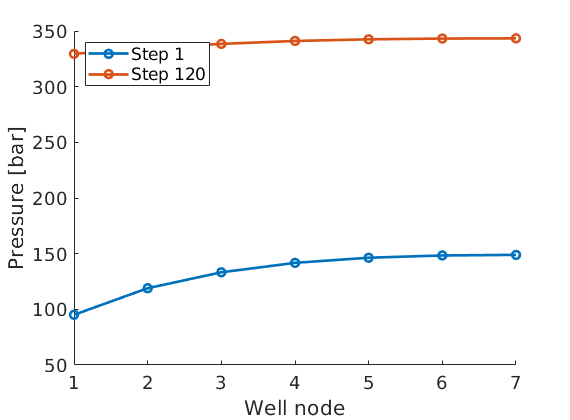
Plot the well-bore pressure in the multisegment well
Plot pressure along wellbore for step 1 and step 120 (final step)
figure, hold all
for k =  [1 120]
    plot([wellSols{k}(2).bhp; wellSols{k}(2).nodePressure(1:6)]/barsa, ...
         '-o', 'LineWidth', 2);
end
legend('Step 1', 'Step 120', 'Location', 'northwest')
set(gca, 'Fontsize', 14), xlabel('Well node'), ylabel('Pressure [bar]')
Launch interactive plotting
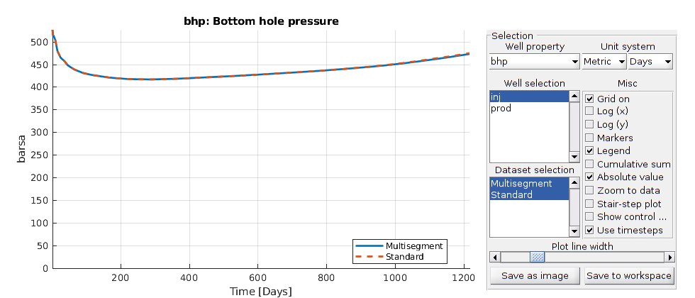
We can compare the two different well models interactively and observe the difference between the two modelling approaches.
plotWellSols({wellSols, wellSolsSimple}, report.ReservoirTime, ...
            'datasetnames', {'Multisegment', 'Standard'});
Show the advancing displacement front
mrstModule add coarsegrid
pg = generateCoarseGrid(G,ones(G.cells.num,1));
figure, h = [];
plotGrid(pg,'FaceColor','none');
plotGrid(G,c,'FaceColor','none','EdgeColor','r');
plotWell(G,[inj; prodS]);
 caxis([0 .5]); view(37.5,34); caxis([0 .5]); axis tight; colorbar, drawnow;
for i=1:numel(states)
    sg = states{i}.s(:,3); inx = sg>1e-5;
    if sum(inx)>0
        delete(h)
        h=plotCellData(G,sg,sg>1e-4,'EdgeAlpha',.01);
        colorbar
    drawnow;
    end
end
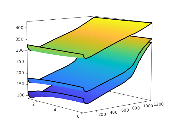
Visualize drawdown in well as function of time
We extract the pressure in all the nodes and visualize this, together with the pressure in the completed reservoir cells as function of time
[xx,tt]=meshgrid(1:6,report.ReservoirTime/day);
pr = cellfun(@(x) x.pressure(c)', states, 'UniformOutput',false);
pa = cellfun(@(x) x(2).nodePressure(7:12)', wellSols, 'UniformOutput',false);
pw = cellfun(@(x) x(2).nodePressure(1:6)', wellSols, 'UniformOutput',false);
figure
hold on
surfWithOutline(xx, tt, vertcat(pr{:})/barsa);
surfWithOutline(xx, tt, vertcat(pa{:})/barsa);
surfWithOutline(xx, tt, vertcat(pw{:})/barsa);
hold off, box on, axis tight
view(50,10), shading interp
set(gca,'Projection','Perspective');
akse = axis();
cax = caxis();
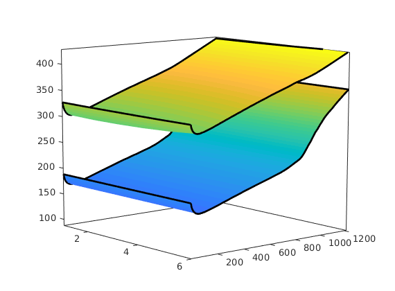
r = cellfun(@(x) x.pressure(c)', statesSimple, 'UniformOutput',false);
pw = cellfun(@(x) x(2).bhp + x(2).cdp', wellSolsSimple, 'UniformOutput',false);
figure
hold on
surfWithOutline(xx, tt, vertcat(pr{:})/barsa);
surfWithOutline(xx, tt, vertcat(pw{:})/barsa);
hold off, box on, axis tight, axis(akse), caxis(cax)
view(50,10), shading interp
set(gca,'Projection','Perspective');

% <html>
% <p><font size="-1
Workflow example for MRST-AD
Generated from simulatorWorkflowExample.m
This example aims to show the complete workflow for creating, running and analyzing a simulation model. Unlike the other examples, we will create all features of the model manually to get a self-contained script without any input files required. The model we setup is a slightly compressible two-phase oil/water model with multiple wells. The reservoir has a layered strategraphy and contains four intersecting faults. Note that this example features a simple conceptual model designed to show the workflow rather than a problem representing a realistic scenario in terms of well locations and fluid physics.
mrstModule add ad-core ad-blackoil ad-props mrst-gui
close all;
Reservoir geometry and petrophysical properties
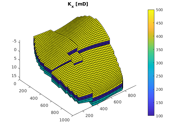
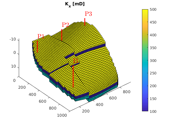
We begin by setting up the grid and rock structures. The grid is created by “makeModel3”, which creates a structured model with intersecting faults. We assume a layered permeability structure with 300, 100, and 500 md in the lower, middle, and top layers. respectively.
% Define grid
grdecl = makeModel3([50, 50, 5], [1000, 1000, 5]*meter);
G = processGRDECL(grdecl);
G = computeGeometry(G);

% Set up permeability based on K-indices
[I, J, K] = gridLogicalIndices(G);

top = K < G.cartDims(3)/3;
lower = K > 2*G.cartDims(3)/3;
middle = ~(lower | top);

px = ones(G.cells.num, 1);
px(lower) = 300*milli*darcy;
px(middle) = 100*milli*darcy;
px(top) = 500*milli*darcy;

% Introduce anisotropy by setting K_x = 10*K_z.
perm = [px, px, 0.1*px];
rock = makeRock(G, perm, 0.3);

% Plot horizontal permeability and wells
figure(1); clf
plotCellData(G, rock.perm(:, 1)/(milli*darcy))
view(50, 50), axis tight
colorbar
title('K_x [mD]')
Adding 5000 artificial cells at top/bottom

Processing regular i-faces
 Found 14964 new regular faces
Elapsed time is 0.012135 seconds.

Processing i-faces on faults
 Found 58 faulted stacks
...
Define wells and simulation schedule
Hydrocarbon is recovered from producers, operating at fixed bottom-hole pressure and perforated throughout all layers of the model. The producers are supported by a single water injector set to inject one pore volume over 10 years (the total simulation length). We also set up a schedule consisting of 5 small control steps initially, followed by 25 larger steps. We keep the well controls fixed throughout the simulation.
simTime = 10*year;
nstep   = 25;
refine  = 5;

% Producers
pv      = poreVolume(G, rock);
injRate = 1*sum(pv)/simTime;
offset  = 10;
W = verticalWell([], G, rock, offset, offset, [],...
                'Name', 'P1', 'comp_i', [1 0], 'Val', 250*barsa, 'Type', 'bhp', 'refDepth', -8);
W = verticalWell(W, G, rock,  offset, floor(G.cartDims(1)/2)+3, [],...
                'Name', 'P2', 'comp_i', [1 0], 'Val', 250*barsa, 'Type', 'bhp', 'refDepth', -8);
W = verticalWell(W, G, rock, offset, G.cartDims(2) - offset/2, [], ...
                'Name', 'P3', 'comp_i', [1 0], 'Val', 250*barsa, 'Type', 'bhp', 'refDepth', -8);
% Injectors
W = verticalWell(W, G, rock, G.cartDims(1)-5, offset, 1,...
                'Name', 'I1', 'comp_i', [1 0], 'Val', injRate, 'Type', 'rate', 'refDepth', -8);

% Compute the timesteps
startSteps = repmat((simTime/(nstep + 1))/refine, refine, 1);
restSteps =  repmat(simTime/(nstep + 1), nstep, 1);
timesteps = [startSteps; restSteps];

% Set up the schedule containing both the wells and the timesteps
schedule = simpleSchedule(timesteps, 'W', W);

% Plot the wells
plotWell(G, W)
axis tight
Set up simulation model
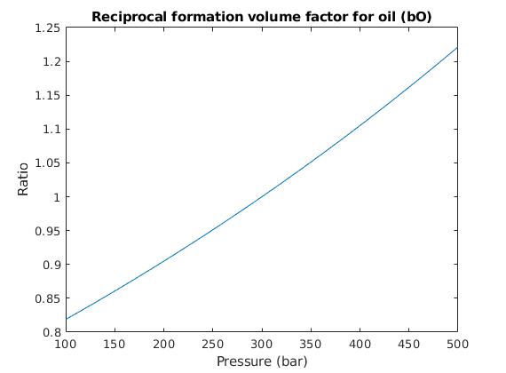
We set up a two-phase oil-water simulation model based on automatic differentiation. The resulting object is a special case of a general three-phase model and to instantiate it, we start by constructing a two-phase fluid structure with properties given for oil and water. Water is assumed to be incompressible, whereas oil has constant compressibility, giving a reciprocal formation volume factor of the form,
. To define this relation, we set the ‘bo’ field of the fluid structure to be an anonymous function that calls the builtin ‘exp’ function with appropriate arguments. Since the fluid model is a struct containing function handles, it is simple to modify the fluid to use alternate functions. We then pass the fundamental structures (grid, rock and fluid) onto the two-phase oil/water model constructor.
% Three-phase template model
fluid = initSimpleADIFluid('mu',    [1, 5]*centi*poise, ...
                           'rho',   [1000, 700]*kilogram/meter^3, ...
                           'n',     [2, 2], ...
                           'cR',    1e-8/barsa, ...
                           'phases', 'wo');

% Constant oil compressibility
c        = 0.001/barsa;
p_ref    = 300*barsa;
fluid.bO = @(p, varargin) exp((p - p_ref)*c);
clf
p0 = (100:10:500)*barsa;
plot(p0/barsa, fluid.bO(p0))
xlabel('Pressure (bar)')
ylabel('Ratio')
title('Reciprocal formation volume factor for oil (bO)')

% Construct reservoir model
gravity reset on
model = TwoPhaseOilWaterModel(G, rock, fluid);
Define initial state
Once we have a model, we need to set up an initial state. We set up a very simple initial state; we let the bottom part of the reservoir be completely water filled, and the top completely oil filled. MRST uses water, oil, gas ordering internally, so in this case we have water in the first column and oil in the second for the saturations.
region = getInitializationRegionsBlackOil(model, 5, 'datum_pressure', p_ref);
state0 = initStateBlackOilAD(model, region);
clf
plotCellData(G, state0.s(:,1))
plotWell(G,W)
view(50, 50), axis tight
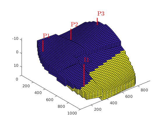
Simulate base case
Using the schedule giving dynamic controls and time steps, the model giving the mathematical description of how to advance the solution, and the initial state of the reservoir, we can simulate the problem. Since the simulation will consume some time, we launch a progress report and a plotting tool for the well solutions (well rates and bottom-hole pressures)
fn = getPlotAfterStep(state0, model, schedule,'view',[50 50], ...
                     'field','s:1','wells',W);
[wellSols, states, report] = ...
   simulateScheduleAD(state0, model, schedule,'afterStepFn',fn);
*****************************************************************
********** Starting simulation:    30 steps,  3650 days *********
*****************************************************************
Preparing model for simulation...
Model ready for simulation...
Preparing schedule for simulation...
Schedule ready for simulation...
Validating initial state...
...
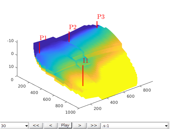
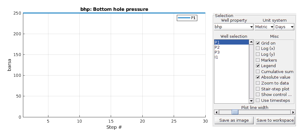
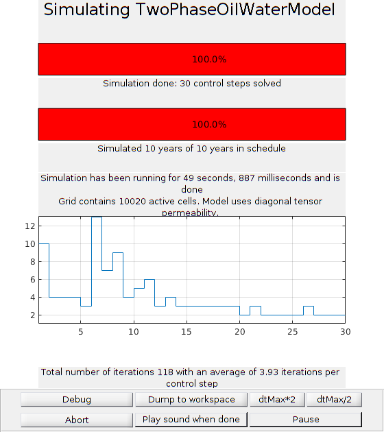
Plot reservoir states
We launch a plotting tool for the reservoir quantities (pressures and saturations, located in states).
figure(1)
plotToolbar(G, states)
view(50, 50);
plotWell(G,W);
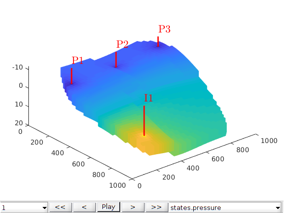
Create an upscaled, coarser model
The fine scale model has approximately 10000 cells. If we want a smaller model we can easily define an upscaled model. Here we set up a simple uniform partition of approximately 50 cells based on the IJK-indices of the grid.
close([2 3]);
mrstModule add coarsegrid
cdims = [5, 5, 2];
p0 = partitionUI(G, cdims);

figp = figure;
CG = generateCoarseGrid(G,p0);
plotCellData(CG,(1:CG.cells.num)', 'EdgeColor', 'none');
plotFaces(CG,1:CG.faces.num,'EdgeColor','k','FaceColor','none');
colormap(.5*colorcube(CG.cells.num)+.5*ones(CG.cells.num,3));
axis tight off
view(125, 55)
title('Straightforward index partition');
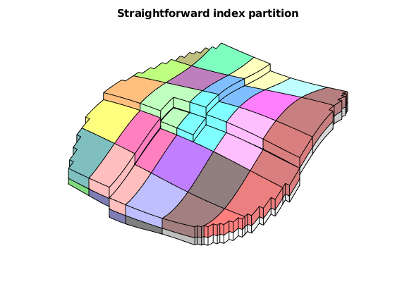
Split blocks over the faultlines
We see that several coarse blocks cross the fault lines. To get hexahedral coarse blocks, we create a grid where the faults act as barriers and apply the “processPartition” routine to split any coarse blocks intersected by faults. Afterwards, we show the new partition and highlight blocks created due to the modification of the fault.
G_fault = makeInternalBoundary(G, find(G.faces.tag > 0));
p = processPartition(G_fault, p0);
plotGrid(G, p ~= p0, 'EdgeColor', 'w', 'FaceColor', 'none')
title('Splitting over fault lines');
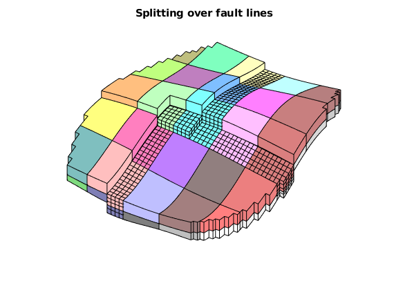
Upscale the model and run the coarser problem
We can now directly upscale the model, schedule, and initial state. By default, the upscaling routine uses the simplest possible options, i.e., harmonic averaging of permeabilities. It is possible to use more advanced options, but for the purpose of this example we will use the defaults. Once we have an upscaled model, we can again simulate the new schedule and observe that the time taken is greatly reduced. For instance, on a Intel Core i7 desktop computer, the fine model takes little under a minute to run, while the upscaled model takes 4 seconds.
clear CG; if ishandle(figp); close(figp); end;
model_c = upscaleModelTPFA(model, p);
G_c    = model_c.G;
rock_c = model_c.rock;

schedule_c = upscaleSchedule(model_c, schedule);
state0_c = upscaleState(model_c, model, state0);

[wellSols_c, states_c] = simulateScheduleAD(state0_c, model_c, schedule_c);
*****************************************************************
********** Starting simulation:    30 steps,  3650 days *********
*****************************************************************
Preparing model for simulation...
Model ready for simulation...
Preparing schedule for simulation...
Schedule ready for simulation...
Validating initial state...
...
Create a second upscaled model with flow-based upscaling
We use the upscaling module to create a tailored upscaled model. This upscaling routine uses a incompressible flow field with the wells of the problem to perform a global upscaling.
mrstModule add incomp agglom upscaling

[~, T_c, W_c] = upscaleTrans(G_c, model.operators.T_all, ...
    'Wells', W, 'bc_method', 'wells', 'fix_trans', true);

model_c2 = upscaleModelTPFA(model, p, 'transCoarse', T_c);
schedule_c2 = schedule;
for i = 1:numel(schedule_c2.control)
    schedule_c2.control(i).W = W_c;
end
[wellSols_c2, states_c2] = simulateScheduleAD(state0_c, model_c2, schedule_c2);
Setting up linear system...                   Elapsed time is 0.037044 seconds.
Solving linear system...                      Elapsed time is 0.027907 seconds.
Computing fluxes, face pressures etc...               Elapsed time is 0.010089 seconds.
Setting up linear system...                   Elapsed time is 0.006289 seconds.
Solving linear system...                      Elapsed time is 0.000382 seconds.
Computing fluxes, face pressures etc...               Elapsed time is 0.002976 seconds.
Warning: Set boundary face trans to zero
*****************************************************************
...
Plot the coarse results, and compare the well solutions
We plot the coarse solutions and compare the well solutions. Note that the upscaling will result in only 70 cells, which is unlikely to give good results with only simple harmonic averaging of permeabilities as used in the first upscaling. The flow-based upscaling gives much better result, but is dependent on having access to the well configuration.
figure(2); clf
plotToolbar(G_c, states_c); plotWell(G, W)
view(50, 50);

figure(3); clf
plotToolbar(G_c, states_c2); plotWell(G, W)
view(50, 50);

plotWellSols({wellSols, wellSols_c, wellSols_c2}, cumsum(schedule.step.val), ...
   'DatasetNames', {'Fine scale', 'Simple upscaling', 'Flow upscaling'}, 'Field', 'qOs');
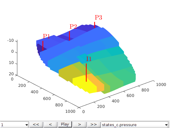
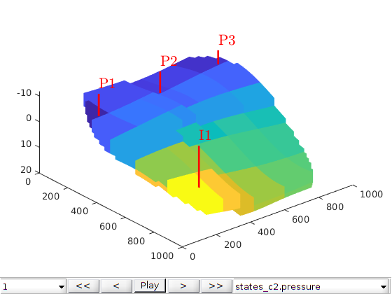
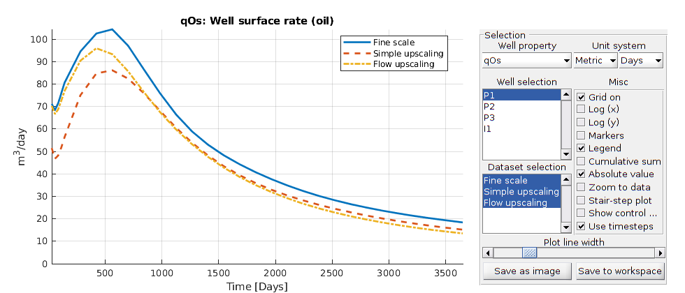
Compute flow diagnostics
As an alternative to looking at well curves, we can also look at the flow diagnostics of the models. Flow diagnostics are simple routines based on time-of-flight and tracer equations, which aim to give a qualitative understanding of reservoir dynamics. Here, we take the end-of-simulation states as a snapshot for both the fine and coarse model and compute time-of-flight and well tracers.
mrstModule add diagnostics
close(3)
D   = computeTOFandTracer(states{end},   G,   rock,   'Wells', schedule.control.W);
D_c = computeTOFandTracer(states_c{end}, G_c, rock_c, 'Wells', schedule_c.control.W);
D_c2 = computeTOFandTracer(states_c2{end}, G_c, rock_c, 'Wells', schedule_c.control.W);
Forward  maximal TOF set to 500.00 years.
Backward maximal TOF set to 496.10 years.
Forward  maximal TOF set to 500.01 years.
Backward maximal TOF set to 493.30 years.
Forward  maximal TOF set to 500.01 years.
Backward maximal TOF set to 495.97 years.
Plot total arrival times
We plot the residence time from injector to producer to separate high-flow regions, shown in dark red, from low-flow or stagnant regions, shown in yellow to white. Since the values vary by several orders of magnitude, we plot the logarithm of the values. We also use the same color axis to ensure that the plots can be compared.
figure(1); clf, cmap=colormap;
hf = plotCellData(G, log10(sum(D.tof, 2))); plotWell(G,W)
view(50, 50); colormap(hot.^.5);
title('Log of total travel time, fine model');
c = caxis();

figure(2); clf
hc = plotCellData(G_c, log10(sum(D_c.tof, 2))); plotWell(G,W)
view(50, 50); colormap(hot.^.5);
title('Log of total travel time, coarse model');
caxis(c)

figure(3); clf
hc2 = plotCellData(G_c, log10(sum(D_c2.tof, 2))); plotWell(G,W)
view(50, 50); colormap(hot.^.5);
title('Log of total travel time, coarse model');
caxis(c)
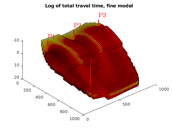
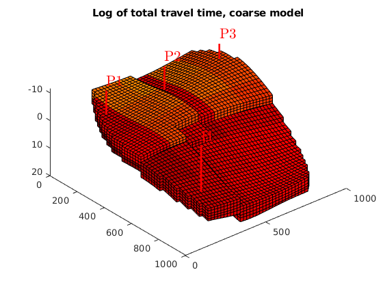
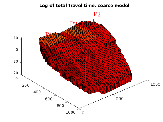
Plot tracer partitioning
We can also look at the tracer partitioning for the producers, showing the drainage regions for the different wells. See the diagnostics module for more examples and more in-depth discussions of how flow diagnostics can be used.
figure(1); delete(hf), colormap(cmap)
plotCellData(G, D.ppart);
title('Drainage regions, fine model');

figure(2); delete(hc), colormap(cmap), caxis auto
plotCellData(G_c, D_c.ppart);
title('Drainage regions, simple upscaled model');

figure(3); delete(hc2), colormap(cmap), caxis auto
plotCellData(G_c, D_c2.ppart);
title('Drainage regions, flow upscaled model');
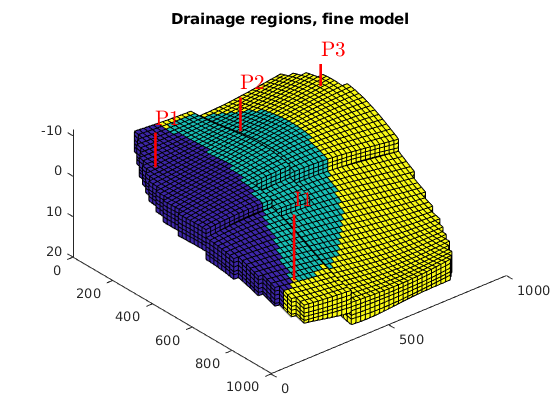
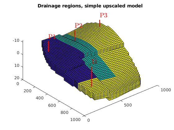
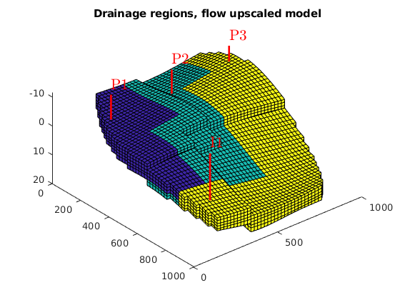
Launch interactive diagnostics tools
We can also examine the diagnostics interactively using the diagnostics viewer.
close all;
interactiveDiagnostics(G, rock, schedule.control.W, 'state', states{end}, 'computeFlux', false, 'name', 'Fine model');
interactiveDiagnostics(G_c, rock_c, schedule_c.control.W, 'state', states_c{end}, 'computeFlux', false, 'name', 'Simple upscaled model');
interactiveDiagnostics(G_c, rock_c, schedule_c.control.W, 'state', states_c2{end}, 'computeFlux', false, 'name', 'Flow upscaled model');
New state encountered, computing diagnostics...
Forward  maximal TOF set to 500.00 years.
Backward maximal TOF set to 496.10 years.
New state encountered, computing diagnostics...
Forward  maximal TOF set to 500.01 years.
Backward maximal TOF set to 493.30 years.
New state encountered, computing diagnostics...
Forward  maximal TOF set to 500.01 years.
...
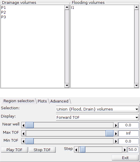
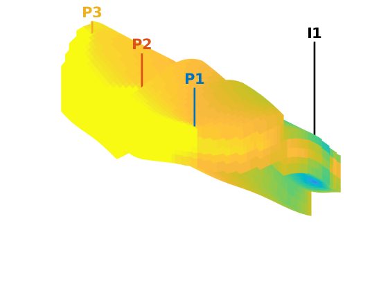

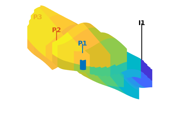

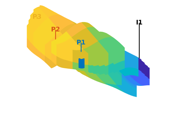
Copyright notice
<html>
% <p><font size="-1
Example demonstrating the two-phase oil-water Egg model
Generated from eggExample.m
This example sets up and runs the Egg model using the two-phase AD solvers. For details on the EggModel and the corresponding ensamble, see Jansen, J. D., et al. “The egg model–a geological ensemble for reservoir simulation.” Geoscience Data Journal 1.2 (2014): 192-195.
mrstModule add ad-core ad-blackoil deckformat
% Realizations can be set to 0 for base cae, or a number between 1 and 100
% for different permeabilities.
realization = 0;
[G, rock, fluid, deck] = setupEGG('realization', realization);
[state, model, schedule, nonlinear] = initEclipseProblemAD(deck, 'G', G, 'TimestepStrategy', 'none');
No converter needed in section 'REGIONS'.
No converter needed in section 'SUMMARY'.
Processing Cells     1 : 18553 of 18553 ... done (0.12 [s], 1.56e+05 cells/second)
Total 3D Geometry Processing Time = 0.120 [s]
No converter needed in section 'REGIONS'.
No converter needed in section 'SUMMARY'.
Ordering well 1 (INJECT1) with strategy "origin".
Ordering well 2 (INJECT2) with strategy "origin".
...
Run simulation
[wellSols, states] = simulateScheduleAD(state, model, schedule, 'NonLinearSolver', nonlinear);
*****************************************************************
********** Starting simulation:   123 steps,  3600 days *********
*****************************************************************
Preparing model for simulation...
Model ready for simulation...
Preparing schedule for simulation...
Schedule ready for simulation...
Validating initial state...
...
Plot the injector BHP and the well oil and water rates
Since the injectors are rate controlled and the producers are pressure controlled, we can plot the quantities that vary. We also plot the water cut.
T = convertTo(cumsum(schedule.step.val), year);
W = schedule.control(1).W;

inj = find(vertcat(W.sign) > 0);
prod = find(vertcat(W.sign) < 0);
bhp = getWellOutput(wellSols, 'bhp', inj);

clf,
plot(T, convertTo(bhp, barsa), 'linewidth', 2)
legend({W(inj).name})
xlabel('Time [years]')
ylabel('Injector bottom-hole pressure [bar]')

orat = getWellOutput(wellSols, 'qOs', prod);
wrat = getWellOutput(wellSols, 'qWs', prod);

figure;
plot(T, convertTo(-orat, meter^3/day), 'linewidth', 2)
legend({W(prod).name})
xlabel('Time [years]')
ylabel('Producer oil-rate [m^3/day]');

figure;
plot(T, convertTo(-wrat, meter^3/day), 'linewidth', 2)
legend({W(prod).name})
xlabel('Time [years]')
ylabel('Producer water-rate [m^3/day]');

figure;
plot(T, abs(wrat)./abs(wrat + orat), 'linewidth', 2)
legend({W(prod).name})
xlabel('Time [years]')
ylabel('Water cut');
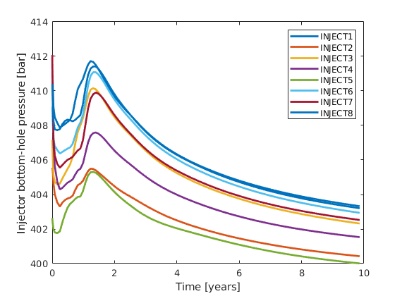
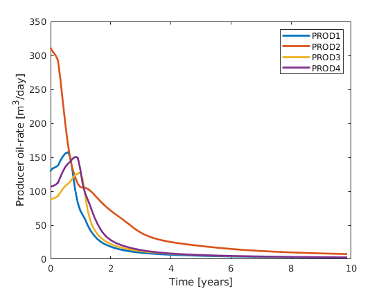
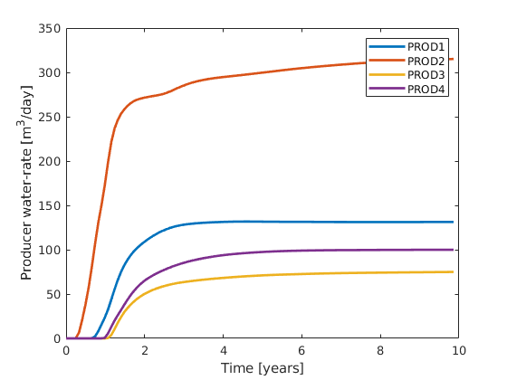
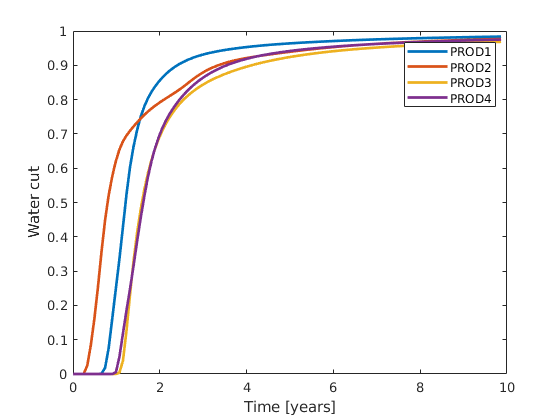
Plot the pressure and water saturation through the simulation
df = get(0, 'DefaultFigurePosition');
h = figure('Position', df.*[1, 1, 2.25, 1]);
for i = 1:numel(states)
    % Plot the pressure
    timestr = formatTimeRange(sum(schedule.step.val(1:i)));
    figure(h); clf
    subplot(1, 2, 1)
    plotCellData(G, states{i}.pressure/barsa, 'EdgeColor', 'none');
    plotWell(G, W(inj), 'fontsize', 12, 'color', 'k')
    plotWell(G, W(prod), 'fontsize', 12, 'color', 'r')
    title(['Reservoir pressure after ', timestr]);
    view(-50, 70);
    axis tight off
    colorbar

    % Plot water saturation
    subplot(1, 2, 2)
    plotCellData(G, states{i}.s(:, 1), 'EdgeColor', 'none');
    plotWell(G, W(inj), 'fontsize', 12, 'color', 'k')
    plotWell(G, W(prod), 'fontsize', 12, 'color', 'r')
    title(['Water saturation after ', timestr]);
    view(-50, 70);
    axis tight off
    colorbar
    caxis([0, 1])
    drawnow
end
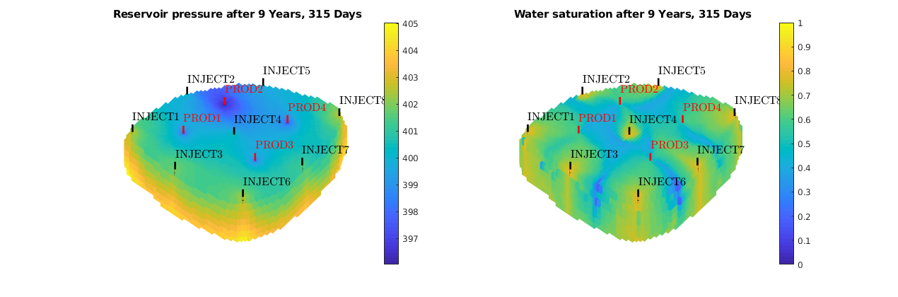
Launch interactive plotting
rstModule add mrst-gui
plotWellSols(wellSols, cumsum(schedule.step.val))

figure;
plotToolbar(G, states)
plotWell(G, W(inj), 'fontsize', 12, 'color', 'k')
plotWell(G, W(prod), 'fontsize', 12, 'color', 'r')

view(-50, 70);
axis tight off

% <html>
% <p><font size="-1
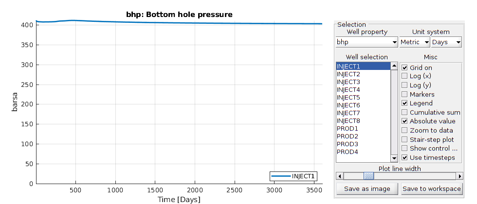
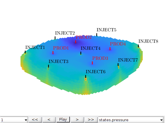
The Odeh Benchmark (SPE1)
Generated from blackoilTutorialSPE1.m
The first SPE project comparing black-oil reservoir simulators was organized by Odeh (1981) and describes a depletion problem with gas injection in a small 10x10x3 reservoir with a producer and an injector placed in diagonally opposite corners. The porosity is uniform and equal 0.3, whereas the permeability is isotropic with values 500, 50, and 200 md in the three layers with thickness 20, 30, and 50 ft. The reservoir is initially undersaturated with a pressure field that is constant in each layer, a uniform mixture of water (Sw = 0.12) and oil (So = 0.88) with no initial free gas (Sg = 0.0) and a constant dissolved gas-oil ratio (Rs ) throughout the model. The problem is specified using an industry-standard input format, and the solution computed by MRST is compared to that of a commercial reservoir simulator (Eclipse 100). The original problem was posed to study ten years of production; herein, we only report and compare solutions for the first 1216 days.
%
% Odeh, A.S. 1981. Comparison of Solutions to a Three-Dimensional Black-Oil
% Reservoir Simulation Problem. J Pet Technol 33 (1): 13–25. SPE-9723-PA.
% http://dx.doi.org/10.2118/9723-PA
%
mrstModule add ad-props deckformat mrst-gui ad-core ad-blackoil
Set up the problem
Because several examples use the SPE1 dataset, the initial setup is delegated to a helper function. See the inside for documentation.
[G, rock, fluid, deck, state] = setupSPE1();

% Determine the model automatically from the deck. It should be a
% three-phase black oil model with gas dissoluton.
model = selectModelFromDeck(G, rock, fluid, deck);

model %#ok, intentional display

% Convert the deck schedule into a MRST schedule by parsing the wells
schedule = convertDeckScheduleToMRST(model, deck);
No converter needed in section 'REGIONS'.
No converter needed in section 'SUMMARY'.
Adding 200 artificial cells at top/bottom

Processing regular i-faces
 Found 550 new regular faces
Elapsed time is 0.001601 seconds.

...
Plot well and permeability
The permeability consists of three layers going from high to low permeability along the z axis. The wells are completed in the upper and lower layer for the injector and producer respectively. To get a well object, we simply process the first control from the schedule.
figure;
plotCellData(G, convertTo(rock.perm(:,1), milli*darcy), ...
             'FaceAlpha', 0.5, 'EdgeAlpha', 0.3, 'EdgeColor', 'k');
plotWell(G, schedule.control(1).W, 'radius',.5); % Pick the only well control present
title('Permeability (mD)')
axis tight, view(35, 40), colorbar('SouthOutside');
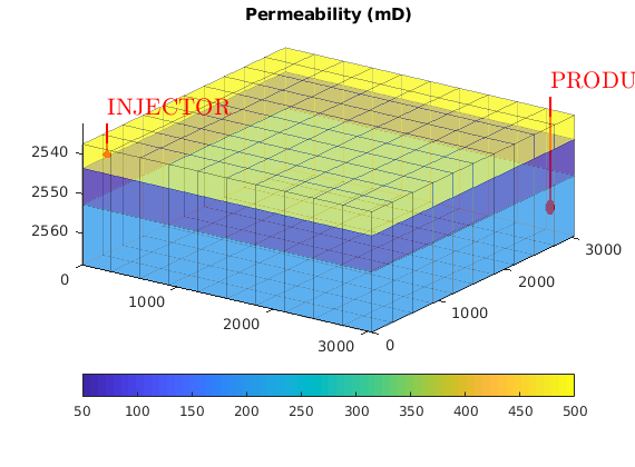
Run the entire schedule
Here, we will run the schedule as it is described in the input file. Note that a schedule is not necessary to solve problems using the fully implicit solver. The function ‘solvefiADI’ from the ‘ad-fi’ module (which implements fully implicit ad solvers without object orientation) is capable of taking a well structure directly and solve for a single time step in a manner similar e.g., to the incompressible MRST solvers. schedule.step.val(1) = 10*year;
nls = NonLinearSolver('useLinesearch', true);
[wellSols, states, report] = simulateScheduleAD(state, model, schedule, 'nonlinearsolver', nls);
*****************************************************************
********** Starting simulation:   120 steps,  1216 days *********
*****************************************************************
Preparing model for simulation...
Model ready for simulation...
Preparing schedule for simulation...
Schedule ready for simulation...
Validating initial state...
...
Plot the well solutions and simulator states
We setup interactive viewers for both well solutions and the reservoir states.
plotWellSols(wellSols, report.ReservoirTime)

figure;
plotToolbar(G, states)
plotWell(G, schedule.control(1).W)
axis tight, view(-10, 60)
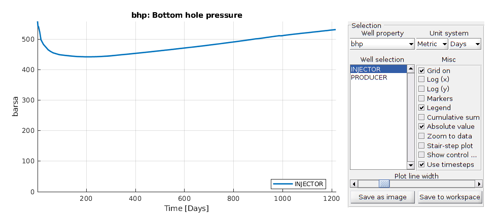
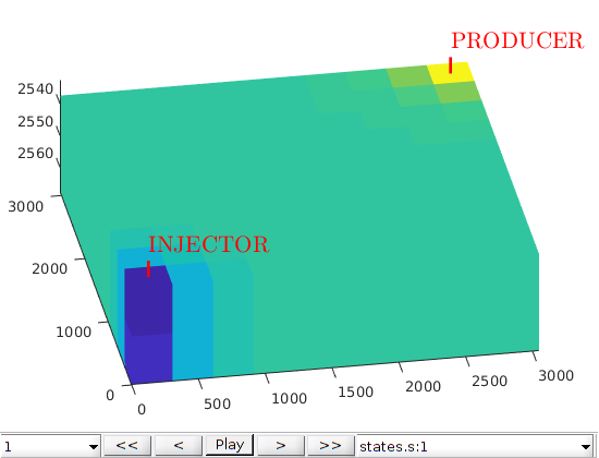
Make plots to compare solution with a commercial simulator
Load summary from binary file and find indices of the producer and injector.
load SPE1_smry

inj = find([wellSols{1}.sign] == 1);
prod = find([wellSols{1}.sign] == -1);

% Since there are zero values in the first step of the summary, we ignore
% the first entry to get better plot axes.
ind = 2:size(smry.data,2);

% Put the well solution data into a format more suitable for plotting
[qWs, qOs, qGs, bhp] = wellSolToVector(wellSols);

% Get timesteps for both the reference and the MRST solution
T = convertTo(cumsum(schedule.step.val), year);
Tcomp =  smry.get(':+:+:+:+', 'YEARS', ind);
Plot producer gas/oil ratio
The most interesting part of the SPE1 case is the gas/oil ratio at the producer. We convert the field units and plot the dimensionless ratio. As should be apparent from the figure, the implicit solver is able to qualitatively reproduce the same outflow profile.
figure(3)
clf
ecl = convertFrom(smry.get('PRODUCER', 'WGOR', ind), 1000*ft^3/stb)';
mrst = qGs(:,prod)./qOs(:,prod);

mrstarg = {'LineWidth', 2};
eclarg = {'ro','MarkerSize',5,'MarkerFaceColor',[.6 .6 .6]};
hold on
plot(T, mrst, mrstarg{:})
plot(Tcomp, ecl, eclarg{:});
legend({'MRST', 'Eclipse'})
xlabel('Time [Years]')
title('Gas rate / Oil rate')
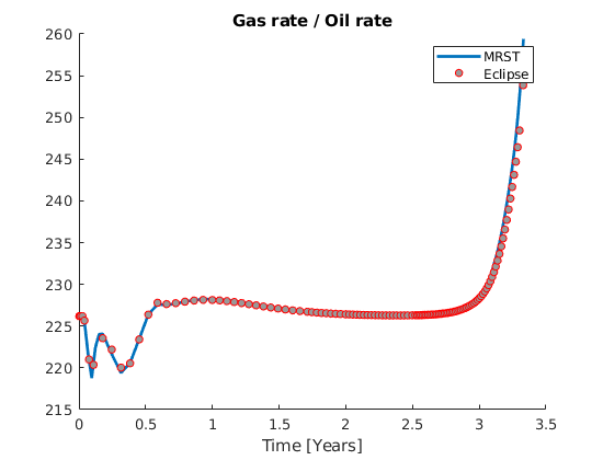
Plot producer bottom-hole pressure
The injector is rate controlled and so the bottom-hole pressure is solved in the implicit loop. Plot it to verify accuracy.
figure(4)
clf
ecl = convertFrom(smry.get('PRODUCER', 'WBHP', ind), psia)';
mrst = bhp(:,prod);
hold on
plot(T,     convertTo(mrst, barsa), mrstarg{:})
plot(Tcomp, convertTo(ecl, barsa), eclarg{:});
legend({'MRST', 'Eclipse'})
xlabel('Time [Years]')
ylabel('bar')
title('Bottom-hole pressure (producer)')
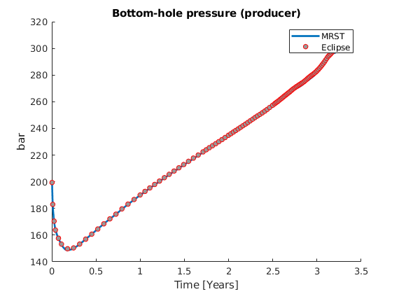
Plot injector bottom-hole pressure
figure(5)
clf
ecl = convertFrom(smry.get('INJECTOR', 'WBHP', ind), psia)';
mrst = bhp(:,inj);
hold on
plot(T,     convertTo(mrst, barsa), mrstarg{:})
plot(Tcomp, convertTo(ecl, barsa),  eclarg{:});
legend({'MRST', 'Eclipse'})
xlabel('Time [Years]')
ylabel('bar')
title('Bottom-hole pressure (injector)')
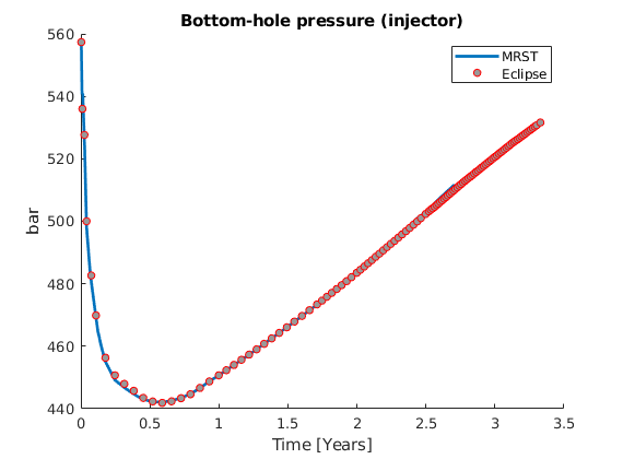
Copyright notice
<html>
% <p><font size="-1
Automated Time-Step Control
Generated from timestepControlDemo.m
The ad-core module offers several options for automatic time-step control. The simplest approach is to run the time steps as prescribed and use a heuristic algorithm to reduce the time step if the number of nonlinear iterations exceeds a prescribed limit; this is commonly referred to as the Appleyard chop. In the modified version, one also monitors the saturation increments and reduces the time step if the saturation changes more than a prescribed limit within a single time step. MRST also offers more a sophisticated time-step control that monitors the convergence of the nonlinear solves and adjusts the time-step so that the number of nonlinear iterations stays close to a prescribed target. In this example, we will use the SPE1 benchmark to demonstrate this time step control.
mrstModule add ad-props deckformat mrst-gui ad-core ad-blackoil
Load and run the SPE1 model
Because several examples use the SPE1 dataset, the initial setup is delegated to a helper function. See the inside for documentation.
[G, rock, fluid, deck, state] = setupSPE1();

% Determine the model automatically from the deck. It should be a
% three-phase black oil model with gas dissoluton.
model = selectModelFromDeck(G, rock, fluid, deck);

model %#ok, intentional display

% Convert the deck schedule into a MRST schedule by parsing the wells
schedule = convertDeckScheduleToMRST(model, deck);

% Run base case
[wellSols, states, report] = simulateScheduleAD(state, model, schedule);
No converter needed in section 'REGIONS'.
No converter needed in section 'SUMMARY'.
Adding 200 artificial cells at top/bottom

Processing regular i-faces
 Found 550 new regular faces
Elapsed time is 0.001781 seconds.

...
Time-step control with iteration targets
Because the SPE1 benchmark uses the same well configuration throughout the entire simulation, we are (relatively) free to choose timesteps. To demonstrate this, we create a simpler schedule consisting of a single very long timestep and then let the time-step control automatically select the length of the individual time steps so that the number of iterations for each step stays close to a prescribed target. We will run four simulations with target values 4, 8, 15, and 25. Use the compressSchedule routine to reduce the schedule to the minimal number of timesteps required to honor the distinct control steps. In this case, we only have a single control step. To get a stable solution, we also need to start with a small time step to get the solver started. Here, we start with a time step of one day and then gradually increase the length of the time step to stay close to our iteration target.
% Reduce to a minimal schedule
schedule_small = compressSchedule(schedule);

% Run all four simulations
rampup = 1*day;
targetIts = [4 8 15 25];
[reports, ws] = deal(cell(numel(targetIts), 1));
for i = 1:numel(targetIts)
    % Set up time selection class
    timestepper = ...
       IterationCountTimeStepSelector('targetIterationCount', targetIts(i),...
                                      'minRelativeAdjustment', sqrt(eps),...
                                      'maxRelativeAdjustment', 4, ...
                                      'firstRampupStep',       rampup, ...
                                      'verbose', true);

    % Instantiate a nonlinear solver with the timestep class as a
    % construction argument.
    nonlinear = NonLinearSolver('timeStepSelector', timestepper, ...
                                'maxiterations', 4*targetIts(i));
    % Solve and store results.
    [ws{i}, ~, reports{i}] = simulateScheduleAD(state, model, schedule_small,...
                        'nonlinearSolver', nonlinear, 'outputMinisteps', true);
end
*****************************************************************
********** Starting simulation:     1 steps,  1216 days *********
*****************************************************************
Preparing model for simulation...
Model ready for simulation...
Preparing schedule for simulation...
Schedule ready for simulation...
Validating initial state...
...
Combine output
We now have reports and solutions for the base case and the cases using automatic time-stepping. We extract the length of each time step from the simulation reports and plot versus time
l = arrayfun(@(x) ['Target: ', num2str(x), ' its'], targetIts, 'UniformOutput', false);
l = horzcat('Base case', l);

wsols = vertcat({wellSols}, ws);

timesteps = cell(numel(reports) + 1, 1);
timesteps{1} = schedule.step.val;
for i = 1:numel(reports)
    % Read out the actually used timesteps
    [~, t] = convertReportToSchedule(reports{i}, schedule_small);
    timesteps{i+1} = t;
end
% Sum up all timesteps to get time at each datapoint
time = cellfun(@cumsum, timesteps, 'UniformOutput', false);

% Plot the timestep lengths
figure;
hold on
c = lines(numel(timesteps));
for i = 1:numel(timesteps);
    plot(time{i}/day, timesteps{i}/day, '-o', 'linewidth', 2, 'color', c(i, :))
    grid on
end
legend(l,'Location','NorthWest')
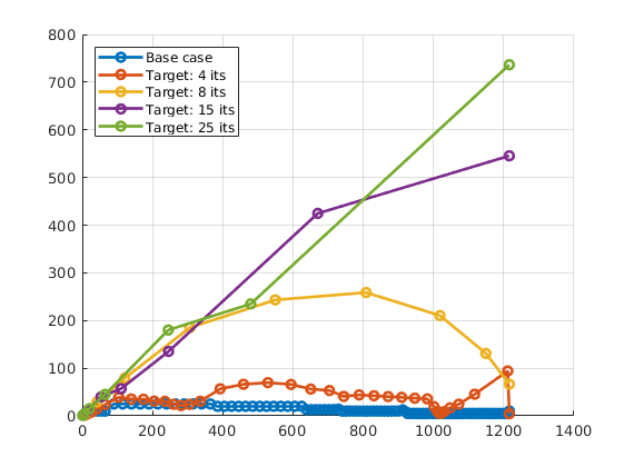
Compare solution accuracy (well curves)
Looking at the various well curves, we see that whereas the water rate and water production is accurately resolved by all simulations, the larger time steps fail to accurately resolve the strong gradients in the oil and gas production as the gas front approaches the producer. On the other hand, using a target of 15 or 25 iterations allows time steps between one and two years, which are extremely, and one should generally not expect that this will give very accurate solutions.
plotWellSols(wsols, time, 'datasetnames', l);
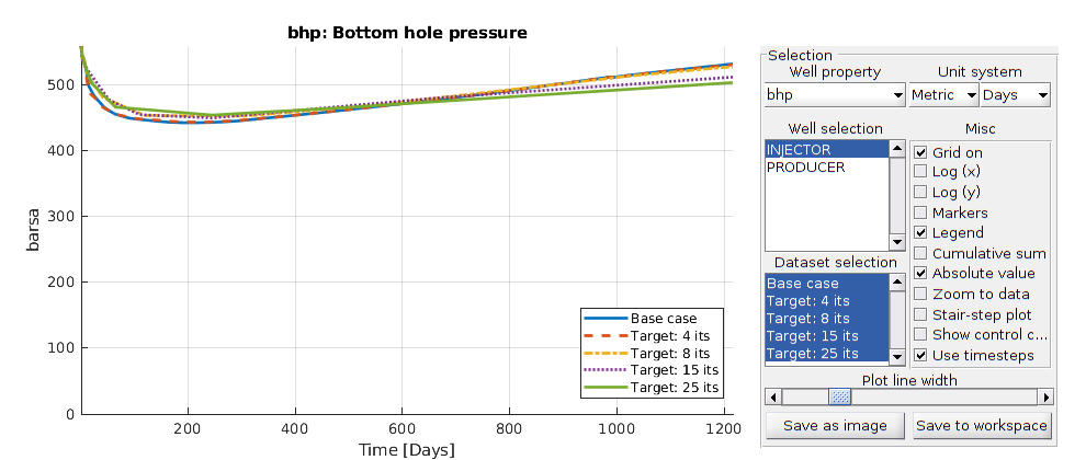
Compare computational efficiency
To get an overall view of the computational cost of each simulation, we need to extract the number of iterations and computational time of each substep. These can be extracted from the report->control step reports.
reps = vertcat({report}, reports);

[iterations, timesteps] = deal(zeros(numel(reps), 1));
for i = 1:numel(reps)
    r = reps{i};
    timesteps(i) = sum(r.SimulationTime);
    for j = 1:numel(reps{i})
        for k = 1:numel(r.ControlstepReports)
            if r.Converged
                iterations(i) = iterations(i) + r.ControlstepReports{k}.Iterations;
            end
        end
    end
end
figure;
bar([iterations, timesteps])
legend('Non-linear iterations', 'Time taken')
set(gca, 'XTicklabel', l)
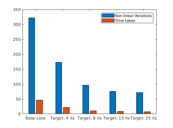
Conclusion
The automatic time-step control enables us to run very large time steps. However, since this will also introduce large errors in the temporal discretization, a reasonable compromise between accuracy and efficiency would most likely be to select an iteration target somewhere in the interval 3 to 8.
Copyright notice
<html>
% <p><font size="-1
Example Simulation of Model One From Tenth SPE CSP
Generated from tenthCSP_Model_I.m
mrstModule add ad-core ad-blackoil ad-props mrst-gui spe10
gravity reset on
Model Geometry
Grid is a 100-by-1-by-20 Cartesian box with equally sized cells of dimensions 25-by-25-by-2.5 feet.
cartDims = [ 100, 1, 20 ];
physDims = cartDims .* [ 25, 25, 2.5 ]*ft;
G = computeGeometry(cartGrid(cartDims, physDims));
Processing Cells    1 : 2000 of 2000 ... done (0.02 [s], 1.06e+05 cells/second)
Total 3D Geometry Processing Time = 0.019 [s]
Petrophysical Properties
Porosity is constant (=0.2) throughout the formation. The permeability distribution is a correlated geostatistically generated field stored in a file supplied by the SPE.
rock = getSPE10_model_1_rock();

clf
plotCellData(G, log10(convertTo(rock.perm(:,1), milli*darcy)))
view(3), axis tight, grid on
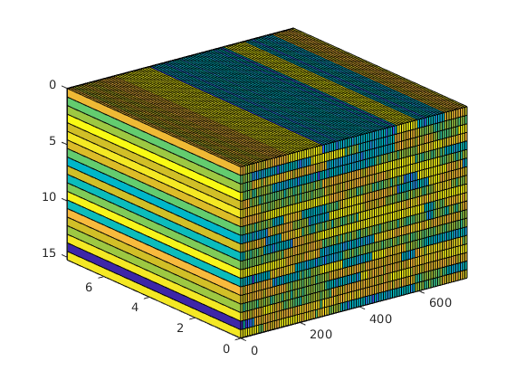
Define Sources and Sinks
Model is produced from a single producer located at the far end of the model (I==100) constrained at a bottom-hole pressure of 95 Psi. There is a single injector at the near end (I==1) providing pressure support. The injector fills the reservoir with 6.97 cubic metres of gas per day. Both wells have an internal diameter of 1 ft.
IJK = gridLogicalIndices(G);
I   = find(IJK{1}(:,1) == 1);
P   = find(IJK{1}(:,1) == G.cartDims(1));  clear IJK

W = addWell([], G, rock, I, 'Comp_i', [ 0, 1 ], 'Type', 'rate', ...
            'Val', 6.97*meter^3/day, 'Radius', (1/2)*ft, 'Dir', 'z', ...
            'Sign', +1, 'Name', 'I', 'refDepth', 0*ft);  clear I

W = addWell(W, G, rock, P, 'Comp_i', [ 1, 1 ], 'Type', 'bhp', ...
            'Val', 95*psia, 'Radius', (1/2)*ft, 'Dir', 'z', ...
            'Sign', -1, 'Name', 'P', 'refDepth', 0*ft);  clear P
Official Benchmark Relative Permeability Data
Build a reduced ECLIPSE-style input deck that contains just enough information to construct relative permeability curves based on the official benchmark data. In particular we use the fact that the relative permeability data is formatted in the same way as ECLIPSE’s ‘SGOF’ keyword data.
kr_deck = getSPE10_model_1_relperm();

clf
plot(kr_deck.PROPS.SGOF{1}(:, 1),            ...
     kr_deck.PROPS.SGOF{1}(:, [2, 3]), '*-', ...
     'LineWidth', 2, 'MarkerSize', 5)
legend({'kr_g', 'kr_o'}, 'Location', 'Best')
xlabel('S_g'), title('Relative Permeability, Model I 10th CSP')
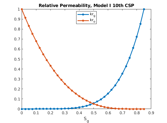
Fluid Properties
The fluids in this simulation model are incompressible and immiscible with constant viscosities. This means we can use MRST’s special purpose fluid constructor initSimpleADIFluid to create the fluid object. We will however need to use sampled relative permeability curves so we do not enter any relative permeability data in this call.
fluid = initSimpleADIFluid('mu'    , [  1, 0.01]*centi*poise, ...
                           'rho'   , [700, 1   ]*kilogram/meter^3, ...
                           'cR'    , 6.0e-5/barsa, ...
                           'phases', 'OG');
Replace the synthetic relative permeability curves created through function initSimpleADIFluid with the real benchmark values.
fluid_kr = assignSGOF(fluid, kr_deck.PROPS.SGOF, struct('sat', 1));
fluid.krG = fluid_kr.krG{1};
fluid.krO = fluid_kr.krOG{1};              clear fluid_kr
Warning: No relperm points found in assignment of SGOF.
The SPE 10 module contains the special purpose function getSPE10_model_1_fluid that performes the above fluid manipulations so one would generally not do this manually.
Form Reservoir Model
This is an incompressible, immiscible oil/gas system.
model = GenericBlackOilModel(G, rock, fluid, 'gravity', gravity, 'disgas', false,...
    'vapoil', false, 'water', false, 'oil', true, 'gas', true);
Initialise Formation
Formation is initially filled with oil and the initial pressure at the top of the model is 100 Psi.
region = getInitializationRegionsBlackOil(model, 0, 'datum_pressure', 100*psia);
state0 = initStateBlackOilAD(model, region);

clf
plotCellData(G, convertTo(state0.pressure, psia))
view(3), colorbar(), axis tight, grid on
xlabel('x'), zlabel('Depth'), title('Initial Pressure Distribution [Psi]')
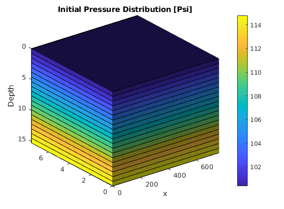
Ten years (3650*day), ramp-up time-steps.
timesteps = [ 0.1, 0.2, 0.3, 0.4, repmat(0.5, [1, 6]), ones([1, 6]), ...
              repmat(2, [1, 5]), repmat(5, [1, 8]), repmat(10, [1, 9]), ...
              repmat(20, [1, 5]), repmat(30, [1, 50]), ...
              repmat(50, [1, 38]) ]*day;

% Set up the schedule containing both the wells and the timesteps
schedule = simpleSchedule(timesteps, 'W', W);
n = getPlotAfterStep(state0, model, schedule, 'view', [50, 50], ...
                      'field', 's:1', 'wells', W);

[wellSols, states, report] = ...
   simulateScheduleAD(state0, model, schedule, 'afterStepFn', fn);

% <html>
% <p><font size="-1
*****************************************************************
********** Starting simulation:   131 steps,  3650 days *********
*****************************************************************
Preparing model for simulation...
Model ready for simulation...
Preparing schedule for simulation...
Schedule ready for simulation...
Validating initial state...
...
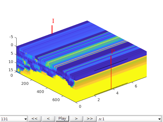
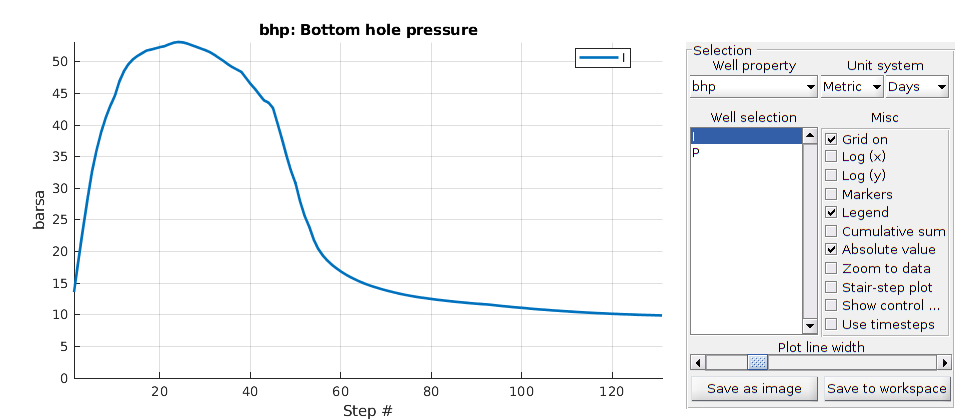
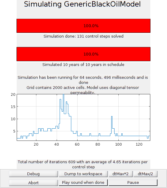
Ninth Comparative Solution Project
Generated from blackoilTutorialSPE9.m
This example runs the model from the SPE9 benchmark, which was posed twenty years ago to compare contemporary black-oil simulators (Killough, 1995). The reservoir is described by a 24 × 25 × 15 grid, having a 10 degree dipping-angle in the x-direction. By current standards, the model is quite small, but contains a few features that will still pose challenges for black-oil simulators. The 25 producers initially operate at a maximum rate of 1500 STBO/D, which is lowered to 100 STBO/D from day 300 to 360, and then raised up again to its initial value until the end of simulation at 900 days. The single water injector is set to a maximum rate of 5000 STBW/D with a maximum bottom-hole pressure of 4000 psi at reference depth. This setup will cause free gas to form after ~100 days when the reservoir pressure is reduced below the original saturation pressure. The free gas migrates to the top of the reservoir. During the simulation most of the wells convert from rate control to pressure control. A second problem is a discontinuity in the water-oil capillary pressure curve, which may cause difficulties in the Newton solver when saturations are changing significantly. In this comprehensive example, we will discuss the various parameters that enter the model and show how to set up state-of-the-art simulation using a CPR preconditioner with algebraic multigrid solver.
mrstModule add ad-blackoil ad-core mrst-gui ad-props deckformat
Set up model
This SPE Comparative Solution Project consists of a water injection problem in a highly heterogenous reservoir. There is one injector and 25 producers. The problem is set up to be solved using a black-oil model. The data set we provide is a modified version of input files belonging to the course in reservoir engineering and petrophysics at NTNU (Trondheim, Norway) and available at http://www.ipt.ntnu.no/~kleppe/pub/SPE-COMPARATIVE/ECLIPSE_DATA/. We have put most of the boilerplate setup into the setupSPE9 function.
[G, rock, fluid, deck, state0] = setupSPE9();

% Determine the model automatically from the deck. It should be a
% three-phase black oil model with gas dissoluton.
model = selectModelFromDeck(G, rock, fluid, deck);

% Show the model
model %#ok, intentional display

% Convert the deck schedule into a MRST schedule by parsing the wells
schedule = convertDeckScheduleToMRST(model, deck);
No converter needed in section 'REGIONS'.
No converter needed in section 'SUMMARY'.
Adding 1200 artificial cells at top/bottom

Processing regular i-faces
 Found 10625 new regular faces
Elapsed time is 0.006496 seconds.

...
Adjust time-step control
To ensure more stable time stepping, we set limits on changes in Rs, pressure, and saturation
model.drsMaxRel = inf;
model.dpMaxRel  = .1;
model.dsMaxAbs  = .1;
Configure linear solver
We proceed to setup a CPR-type solver, using the AGMG linear solver as the multigrid preconditioner. The CPR preconditioner attempts to decouple the fully implicit equation set into a pressure component and a transport component. The pressure is mathematically elliptic/parabolic in nature, and multigrid is well suited for solving these highly coupled, challenging problems. The remainder of the linear system, corresponding to the hyperbolic part of the equations is localized in nature and is primarily concerned with moving the saturation between neighboring grid blocks. Setting up a preconditioner is not strictly required to solve this problem, as the 9000 cells for a three-phase system results in linear systems with 27000 unknowns (one equation per phase, per cell). However, it does improve the solution speed and is required for larger cases, where Matlab’s standard linear solvers scale poorly.
try
    mrstModule add agmg
    pressureSolver = AGMGSolverAD();
catch
    pressureSolver = BackslashSolverAD();
end
linsolve = CPRSolverAD('ellipticSolver', pressureSolver, 'tolerance', 1e-3, 'relativeTolerance', 1e-5);
No module mapping found for
  * agmg
Plot the rock permeability
The SPE9 data set has an anisotropic, inhomogenous permeability field. The vertical permeability is 1/10th of the horizontal values. We plot the permeability using a log10 transform to better see the contrast.
v = [15, 30];
[G, rock] = deal(model.G, model.rock);

clf
K = convertTo(rock.perm(:,1), milli*darcy);
plotCellData(G, log10(K)); view(v), axis tight, box on
set(gca,'Projection','Perspective');
colorbarHist(K, [.01 1e4], 'South', 51, true);
title('SPE9 Horizontal permeability');
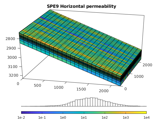
Plot the grid porosity
clf
plotCellData(G, rock.poro), view(v), axis tight, box on
set(gca,'Projection','Perspective');
colorbarHist(rock.poro, [.06 .18], 'South',31);
title('SPE9 Porosity');
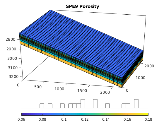
Plot a single vertical set of cells
While the grid is structured, the grid has varying cell size along the vertical axis. To show this in detail, we plot the porosity in a single column of cells. We get the underlying logical grid and extract the subset corresponding to the first column (upper left corner of the grid). By using axis equal we see the actual aspect ratio of the cells.
[ii, jj] = gridLogicalIndices(G);
plotGrid(G, ii==1 & jj==1, 'FaceColor','none','EdgeColor','w');
set(gca,'Position',[.05 .2 .8 .73]); axis off, title('');
axes('Position',[.7 .6 .3 .4]);
plotCellData(G, rock.poro, ii == 1 & jj == 1)
axis equal tight off, view(v)
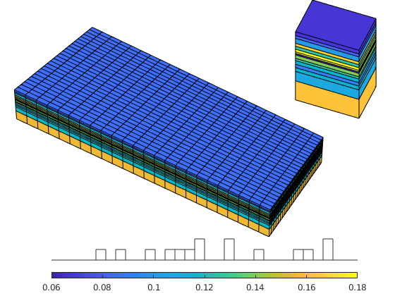
Plot initial saturation of oil and water
Initially, the reservoir does not contain free gas. We plot the initial saturations using the RGB plotting feature, where a three column matrix sent to plotCellData is interpreted column wise as fractions of red, green and blue respectively. Since MRST convention is to order the phases in the order WOG we need to permute the column index slightly to get red oil, blue water and green gas.
s = state0.s(:, [2, 3, 1]);
clf
plotCellData(G, s)
axis tight off; view(v)
set(gca,'Projection','Perspective');

% Add ternary colorbar
axes('Position',[.15 .12 .15 .15]);
patch('Vertices', [0 0; 2 0; 1 2*sin(pi/3)], 'Faces',1:3, ...
    'FaceVertexCData', [0 0 1; 1 0 0; 0 1 0],'FaceColor','interp');
text(0,0,'W','HorizontalAlignment','right');
text(2,0,'O','HorizontalAlignment','left');
text(1,2*sin(pi/3)+.1,'G','HorizontalAlignment','center');
axis tight off
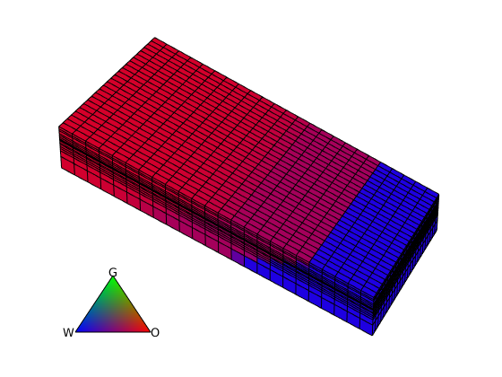
Examine gas dissolved in oil phase
Even though there is no free gas initially, there is significant amounts of gas dissolved in the oil phase. The dissolved gas will bubble into free gas when the pressure drops below the bubble point pressure. For a given pressure there is a fixed amount of gas that can be dissolved in the black-oil instantanous dissolution model. To illustrate how saturated the initial conditions are, we plot the function
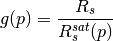
I.e. how close the oil phase is to being completely saturated for the current pressure. A value near one means that the liquid is close to saturated and any values above one will immediately lead to free gas appearing in the simulation model. As we can see from the figure, free gas will appear very quickly should the pressure drop.
Rs_sat = model.fluid.rsSat(state0.pressure);
Rs = state0.rs;

clf
plotCellData(G, Rs./Rs_sat)
axis tight off; colorbar, view(v)
set(gca,'Projection','Perspective');
title('Fraction of maximum gas saturation in oil phase - g(p)');
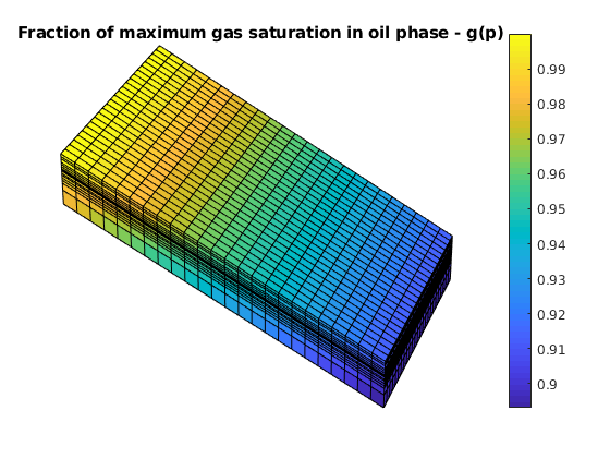
Plot the wells
Since there is a large number of wells, we plot the wells without any labels and simply color the injector in blue and the producers in red.
W = schedule.control(1).W;
sgn = [W.sign];
clf
plotGrid(G, 'FaceColor', 'none')
plotWell(G, W(sgn>0), 'fontsize', 0, 'color', 'b')
plotWell(G, W(sgn<0), 'fontsize', 0, 'color', 'r')
axis tight off; view(v)
set(gca,'Projection','Perspective');
Examine the schedule
The simulation schedule consists of three control periods. All 26 wells are present during the entire simulation, but their prescribed rates will change. The injector is injecting a constant water rate, while the producers all produce a constant oil rate, letting bottom hole pressures and gas/water production vary. Since all producers have the same controls, we can examine PROD2 in detail. We plot the controls, showing that the well rate drops sharply midway during the simulation
wno = find(strcmp({schedule.control(1).W.name}, 'PROD2'));

% Extract controls for all timesteps
P = arrayfun(@(ctrl) schedule.control(ctrl).W(wno).val, schedule.step.control);
T = cumsum(schedule.step.val);
stairs(T/year, convertTo(-P, stb/day), 'o-k','MarkerSize',6,'MarkerFaceColor',[.6 .6 .6])
set(gca,'FontSize',12)
xlabel('Time (years)')
title('Controls for PROD2: oil rate [stb/day]')
set(gca,'YLim',[0 1600]);
Examine well limits
Note that the well controls are not the only way of controlling a well. Limits can be imposed on wells, either due to physical or mathematical considerations. In this case, fixed oil rate is the default setting, but the well will switch controls if the pressure drops below a threshold. This is found in the lims field for each well. Since this is a producer, the bhp limit is considered a lower limit, whereas a bhp limit for an injector would be interpreted as a maximum limit to avoid either equipment failure or formation of rock fractures.
clc
disp(['Well limits for ', schedule.control(1).W(wno).name, ':'])
disp(schedule.control(1).W(wno).lims)
Well limits for PROD2:
    orat: -0.0028
    wrat: -Inf
    grat: -Inf
    lrat: -Inf
     bhp: 6.8948e+06
     thp: 0
Plot relative permeability curves
For a three-phase model we have four relative permeability curves. One for both gas and water and two curves for the oil phase. The oil relative permeability is tabulated for both water-oil and oil-gas systems, and as we can see from the following plot, this gives a number of kinks that will tend to pose challenges for the Newton solver.
f = model.fluid;
s = (0:0.01:1)';

figure;
plot(s, f.krW(s), 'linewidth', 2)
grid on
xlabel('Water saturation');
title('Water relative permeability curve')
ylabel('k_r')

figure;
plot(s, [f.krOW(s), f.krOG(s)], 'linewidth', 2)
grid on
xlabel('Oil saturation');
legend('Oil-Water system', 'Oil-Gas system', 'location', 'northwest')
title('Oil relative permeability curves')
ylabel('k_r')

figure;
plot(s, f.krG(s), 'linewidth', 2)
grid on
xlabel('Gas saturation');
title('Gas relative permeability curve')
ylabel('k_r')
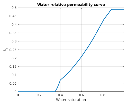
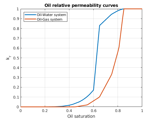
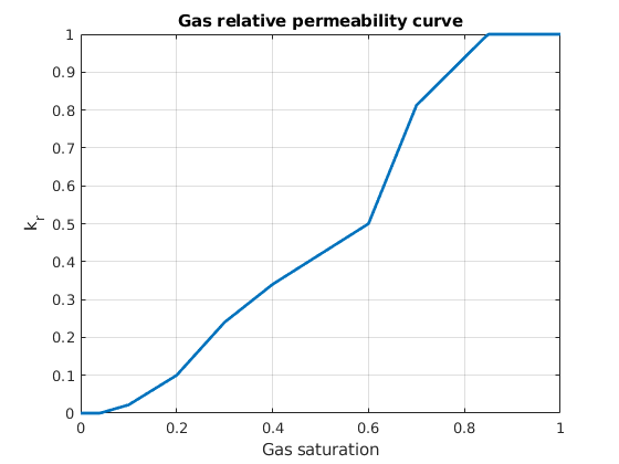
Plot three-phase relative permeability
When all three phases are present simultaneously in a single cell, we need to use some functional relationship to combine the two-phase curves in a reasonable manner, resulting in a two-dimensional relative permeability model. Herein, we use a simple linear interpolation, which is also the default in Eclipse
close all

[x, y] = meshgrid(s);
krO = zeros(size(x));

for i = 1:size(x, 1)
    xi = x(i, :);
    yi = y(i, :);
    [~, krO(i, :), ~] = model.relPermWOG(xi, 1 - xi - yi, yi, f);
end
figure;
krO(x+y>1)=nan;
surfl(x, y, krO), shading interp
xlabel('sW')
ylabel('sG')
title('Oil relative permeability')
view(150, 50); axis tight, camlight headlight
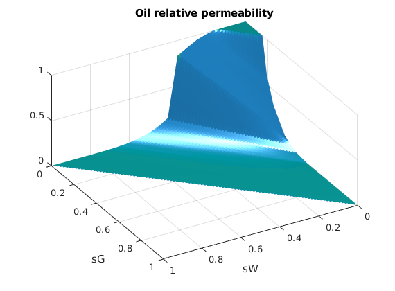
Plot capillary pressure curves
SPE9 contains significant capillary pressure, making the problem more nonlinear as the flow directions and phase potential gradients are highly saturation dependent. Again we have two curves, one for the contact between oil and gas and another for the water-oil contact.
close all
figure;
[ax, l1, l2] = plotyy(s, f.pcOG(s), s, f.pcOW(1 - s));
set([l1, l2], 'LineWidth', 2);
grid on
legend('Oil-Gas capillary pressure', 'Oil-Water capillary pressure', 'location', 'southeast')
xlabel('Oil saturation (Two phase)')
Plot compressibility
The black-oil model treats fluid compressibility through tabulated functions often referred to as formation volume factors (or B-factors). To find the mass of a given volume at a specific reservoir pressure
, we write
where
refers to either the phase, V_R the volume occupied at reservoir conditions and
is the surface / reference density when the B-factor is 1.
Note that MRST by convention only uses small b to describe fluid models. The relation between B and b is simply the reciprocal
and will be calculated when needed.
We begin by plotting the B-factors/compressibility for the water and gas phases. Note that the water compressibility is minimal, as water is close to incompressible in most models. The gas compressibility varies several orders of magnitude. The rock compressibility is included as well. Rock compressibility is modelling the poroelastic expansion of the pore volume available for flow. As the rock itself shrinks, more fluid can fit inside it. Note that although the curves shown in this particular case are all approximately linear, there is no such requirement on the fluid model.
pressure = (50:10:500)'*barsa;

close all
figure;
plot(pressure/barsa, 1./f.bW(pressure), 'LineWidth', 2);
grid on
title('Water formation volume factor')
ylabel('B_w')
xlabel('Pressure [bar]');

figure;
plot(pressure/barsa, 1./f.bG(pressure), 'LineWidth', 2);
grid on
title('Gas formation volume factor')
ylabel('B_g')
xlabel('Pressure [bar]');

figure;
plot(pressure/barsa, f.pvMultR(pressure), 'LineWidth', 2);
grid on
title('Rock compressibility')
ylabel('1 + c_r (p - p_s)')
xlabel('Pressure [bar]');
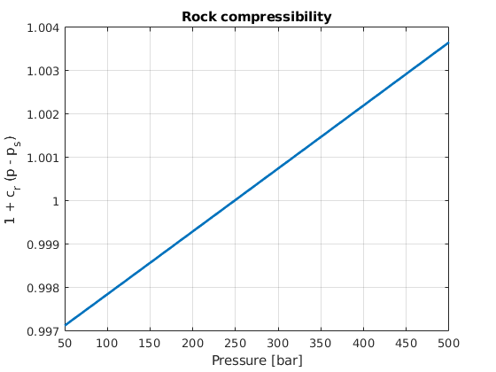
Plot oil compressibility
Since we allow the gas phase to dissolve into the oil phase, compressibility does not only depend on the pressure: The amount of dissolved gas will also change how much the fluid can be compressed. We handle this by having saturated and undersatured tables for the formation volume factors (FVF). This is reflected in the figure: Unsaturated FVF curves will diverge into from the main downwards sloping trend into almost constant curves sloping downwards. Physically, the undersaturated oil will swell as more gas is being introduced into the oil, increasing the volume more than the pressure decreases the volume of the oil itself. When the oil is completely saturated, the volume decrease is due to the gas-oil mixture itself being compressed.
rs = 0:25:320;
[p_g, rs_g] = meshgrid(pressure, rs);
rssat = zeros(size(p_g));
for i = 1:size(p_g, 1)
    rssat(i, :) = f.rsSat(p_g(i, :));
end

saturated = rs_g >= rssat;
rs_g0 = rs_g;
rs_g(saturated) = rssat(saturated);

figure
plot(p_g'/barsa, 1./f.bO(p_g, rs_g, saturated)', 'LineWidth', 2)
grid on
title('Oil formation volume factor')
ylabel('B_o')
xlabel('Pressure [bar]')
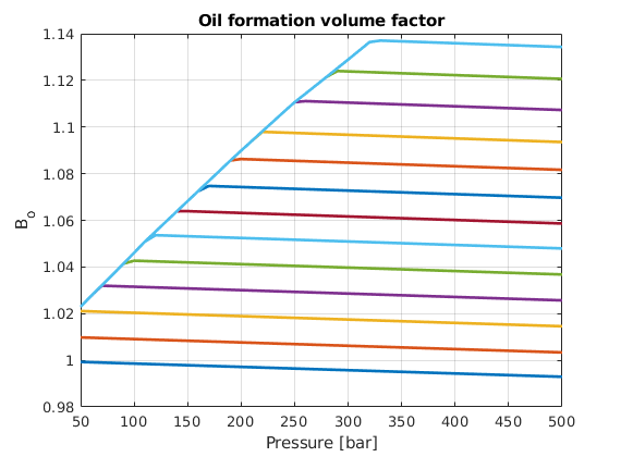
Plot the viscosity
The viscosity can also depend on the pressure and dissolved components in a similar manner as the compressibility. Again, we note that the water phase is unaffected by the pressure, the gas changes viscosity quite a bit. As with
, the oil viscosibility depends more on the amount of dissolved gas than the pressure itself and we have undersatured tables to show.
SPE9 only allows gas to dissolve into oil, and not the other way around. Generally, the black-oil model is a pseudo-compositional model where both gas in oil (
) and oil in gas (
) can be included.
close all
figure;
plot(pressure/barsa, f.muW(pressure), 'LineWidth', 2);
grid on
title('Water viscosity')
ylabel('\mu_w')
xlabel('Pressure');
ylim([0, 1.5e-3])

figure;
plot(pressure/barsa, f.muG(pressure), 'LineWidth', 2);
grid on
title('Gas viscosity')
ylabel('\mu_g')
xlabel('Pressure');

figure;
plot(p_g'/barsa, f.muO(p_g, rs_g, saturated)', 'LineWidth', 2)
grid on
title('Oil viscosity')
ylabel('\mu_o')
xlabel('Pressure')
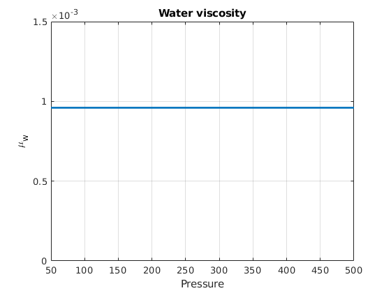
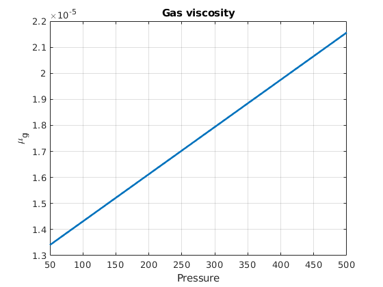
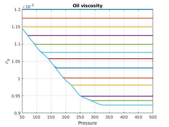
Simulate the schedule
We run the schedule. We provide the initial state, the model (containing the black oil model in this case) and the schedule with well controls, and control time steps. The simulator may use other timesteps internally, but it will always return values at the specified control steps.
close all
model.verbose = false;
fn = getPlotAfterStep(state0, model, schedule, ...
    'plotWell', false, 'plotReservoir', false);
[wellsols, states, reports] =...
    simulateScheduleAD(state0, model, schedule, ...
                       'LinearSolver', linsolve, 'afterStepFn', fn);
*****************************************************************
********** Starting simulation:    35 steps,   900 days *********
*****************************************************************
Preparing model for simulation...
Model ready for simulation...
Preparing schedule for simulation...
Schedule ready for simulation...
Validating initial state...
...
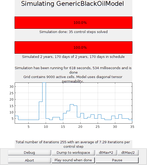
Launch interactive plot tool for well curves
The interactive viewer can be used to visualize the wells and is the best choice for interactive viewing.
plotWellSols(wellsols, cumsum(schedule.step.val))
h = gcf;
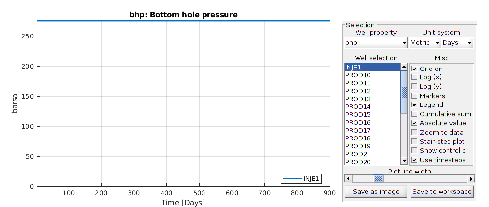
Load comparison data from commercial solver
To validate the simulator output, we load in a pre-run dataset from a industry standard commercial solver run using the same inputs.
addir = mrstPath('ad-blackoil');
compare = fullfile(addir, 'examples', 'spe9', 'compare');
smry = readEclipseSummaryUnFmt(fullfile(compare, 'SPE9'));

compd = 1:(size(smry.data, 2));
Tcomp =  smry.get(':+:+:+:+', 'YEARS', compd);
Reading info from roughly 38 ministeps:  100%
Actual number of ministeps: 37
Set up plotting functions
We will plot the timesteps with different colors to see the difference between the results clearly.
if ishandle(h)
    close(h);
end
T = convertTo(cumsum(schedule.step.val), year);

mrstplot = @(data) plot(T, data, '-b', 'linewidth', 2);
compplot = @(data) plot(Tcomp, data, 'ro', 'linewidth', 2);
Plot two different producers
We plot the bottom-hole pressures for two somewhat arbitrarily chosen producers to show the accuracy of the pressure.
figure;
names = {'PROD13', 'PROD18'};
nn = numel(names);
for i = 1:nn

    name = names{i};

    comp = convertFrom(smry.get(name, 'WBHP', compd), psia)';
    mrst = getWellOutput(wellsols, 'bhp', name);

    subplot(nn, 1, i)
    hold on
    mrstplot(mrst);
    compplot(comp);
    title(name)
    axis tight
    grid on

    xlabel('Time (years)')
    ylabel('Pressure (Pa)')
end
legend({'MRST', 'ECLIPSE'})
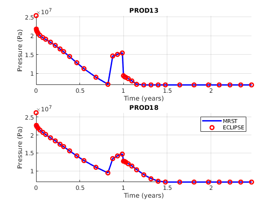
Plot the gas production rate
We plot the gas production rate (at surface conditions).
figure;

for i = 1:nn
    name = names{i};
    comp = convertFrom(smry.get(name, 'WGPR', compd), 1000*ft^3/day);
    mrst = abs(getWellOutput(wellsols, 'qGs', name));

    subplot(nn, 1, i)
    hold on
    mrstplot(mrst);
    compplot(comp);
    title(name)
    axis tight
    grid on

    xlabel('Time (years)')
    ylabel('Gas rate (m^3/s)')
end
legend({'MRST', 'ECLIPSE'})
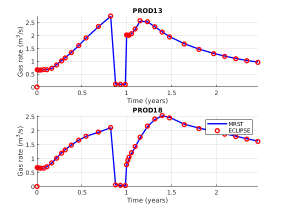
Changing controls
We saw earlier that all wells are initially rate controlled, but in practice a large number of wells will switch controls during the simulation. To show how each well changes throughout the simulation, we will plot indicators per well as a colorized matrix. From this we can clearly see that: - The injector switched immediately to BHP controls and stays there throughout the simulation (Well #1) - The producers are mostly rate controlled in the beginning and mostly BHP controlled at the end as a result of the average field pressure dropping during the simulation as mass is removed from the reservoir. - The period with very low controls at 1 year is easy to see.
isbhp = @(ws) arrayfun(@(x) strcmpi(x.type, 'bhp'), ws);
ctrls = cellfun(isbhp, wellsols, 'UniformOutput', false);
ctrls = vertcat(ctrls{:});

nw = numel(wellsols{1});
nstep = numel(wellsols);

X = repmat(0:nw, nstep, 1)+.5;
Y = repmat(convertTo(convertFrom(T, year), day), 1, nw+1);
C = double(ctrls); C=C(:,[1:end end]);
clf
pcolor(X, Y, C); view(90, 90); axis tight
set(gca,'XTick',[],'FontSize',12);
ylabel('Time (days)')
text((X(1,2:end)+X(1,1:end-1))/2, Y(1,2:end)-5, {wellsols{1}.name},...
    'HorizontalAlignment','right','FontSize',8);
colormap(.55*lines(2)+.45*ones(2,3))
set(colorbar,'Ytick',[.25 .75],'YTickLabel',{'rate','bhp'})

Plot pressure before and after schedule
We plot the pressure after the very first timestep alongside the pressure after the final timestep. By scaling the color axis by the minimum of the final state and the maximum of the first state, we can clearly see how the pressure has dropped due to fluid extraction.
h1 = figure;
h2 = figure;

p_start = states{1}.pressure;
p_end = states{end}.pressure;
cscale = convertTo([min(p_end), max(p_start)],barsa);

figure(h1); clf;
plotCellData(G, convertTo(p_start,barsa))
axis tight; colorbar, view(v), caxis(cscale);
title('Pressure after first timestep')

figure(h2); clf;
plotCellData(G, convertTo(p_end,barsa))
axis tight; colorbar, view(v), caxis(cscale);
title('Pressure after final timestep')
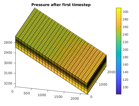
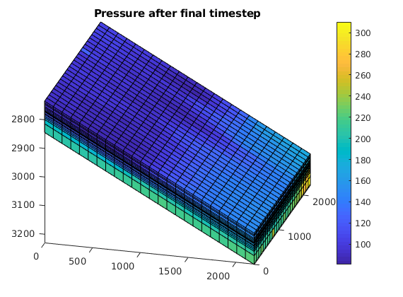
Plot free gas
Since the pressure has dropped significantly and we know that gas is being produced from the initially nearly saturated reservoir, we will look at the free gas. We consider the initial and the last state and use the same coloring.
sg0 = state0.s(:, 3);
sg = states{end}.s(:, 3);
cscale = [0, max(sg)];

figure(h1); clf;
plotCellData(G, sg0)
axis tight off; colorbar; view(v); caxis(cscale);
title('Free gas after first timestep')

figure(h2); clf;
plotCellData(G, sg)
axis tight; colorbar, view(v), caxis(cscale);
title('Free gas after final timestep')
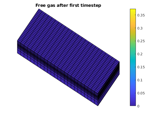
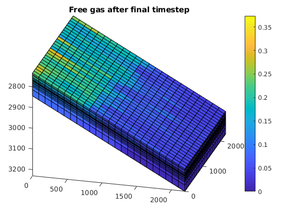
Plot dissolved gas
Since we did not inject any gas, the produced and free gas must come from the initially dissolved gas in oil (
). We plot the values before and after the simulation, scaling the color by the initial values. Note that the
values are interpreted as the fraction of gas present in the oil phase. As the fraction is calculated at standard conditions, the
value is typically much larger than 1. We weight by oil saturations to obtain a reasonable picture of how the gas in oil has evolved. Plotting just the
value is not meaningful if
is small.
gasinoil_0 = states{1}.rs.*states{1}.s(:, 2);
gasinoil = states{end}.rs.*states{end}.s(:, 2);
cscale = [0, max(gasinoil_0)];

figure(h1); clf;
plotCellData(G, gasinoil_0)
axis tight; colorbar; view(v); caxis(cscale);
title('Gas in after first timestep')

figure(h2); clf;
plotCellData(G, gasinoil)
axis tight; colorbar; view(v); caxis(cscale);
title('Gas in oil after final timestep')
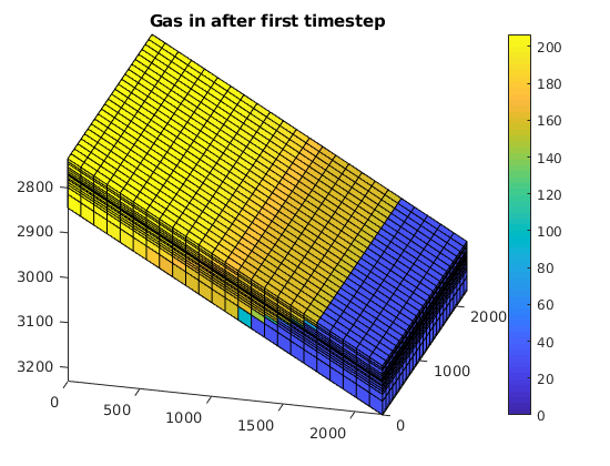
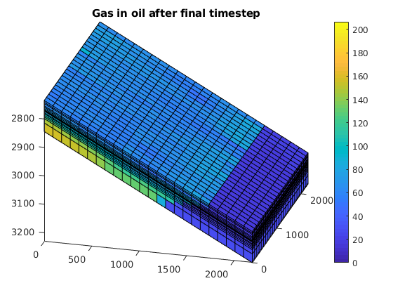
Plot phase distribution
s0 = states{1}.s(:, [2, 3, 1]);
s = states{end}.s(:, [2, 3, 1]);

figure(h1); clf;
plotCellData(G, s0)
axis tight; view(v)
title('Phase distribution after first timestep')

figure(h2); clf;
plotCellData(G, s)
axis tight; view(v)
title('Phase distribution after final timstep')
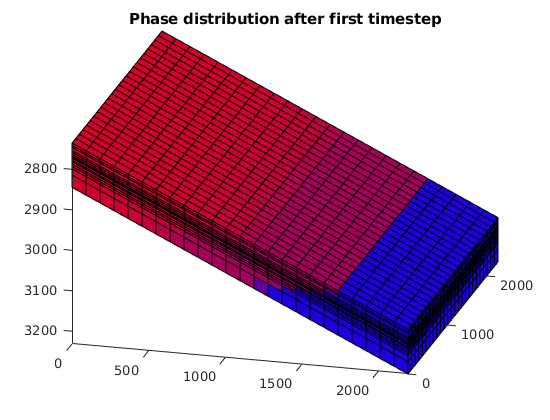
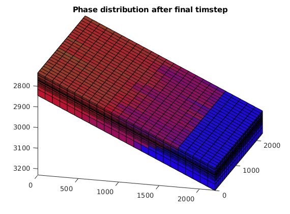
Copyright notice
<html>
% <p><font size="-1