Introduction
exploreCapacity is a demonstration tool for rapid exploration of storage capacities of geological formations in the Norwegian North Sea. It shows how different factors such as aquifer geometry, temperature and pressure regime, rock and fluid properties may affect the final estimate, based on the methodology described in this article.
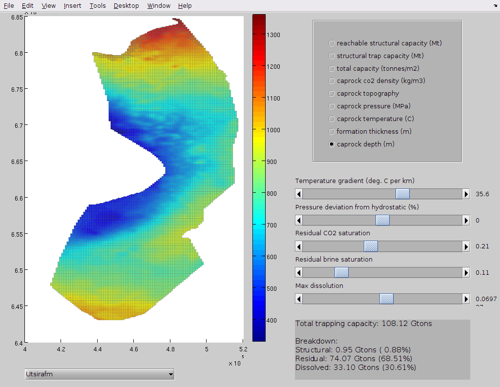
After the user has chosen a geological formation and specified the involved parameters, an estimate of total trapping capacity is provided, broken down by trapping mechanism (structural, residual or dissolution trapping).
The tool is intended to be used for demonstrational and educational purposes, as the data involved is too limited to predict actual capacity with any confidence.
Launching the applicationFirst, ensure that the geological datasets have been downloaded. This can be done in a semi-automatic fashion by launching the graphical dataset download manager as follows: mrstDatasetGUI; Choose the The demonstration tool itself can be launched by ensuring the mrstModule add co2lab % ensure that the co2lab module is loaded exploreCapacity; % run the application The NB: In release var.CO2 = CO2props('sharp_phase_boundary', true);
|
|
|
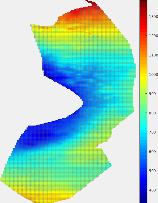
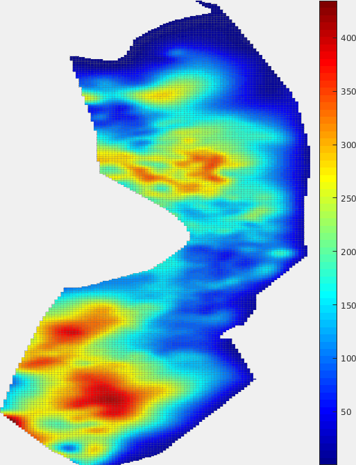
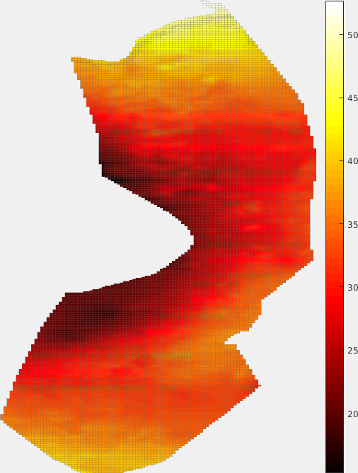
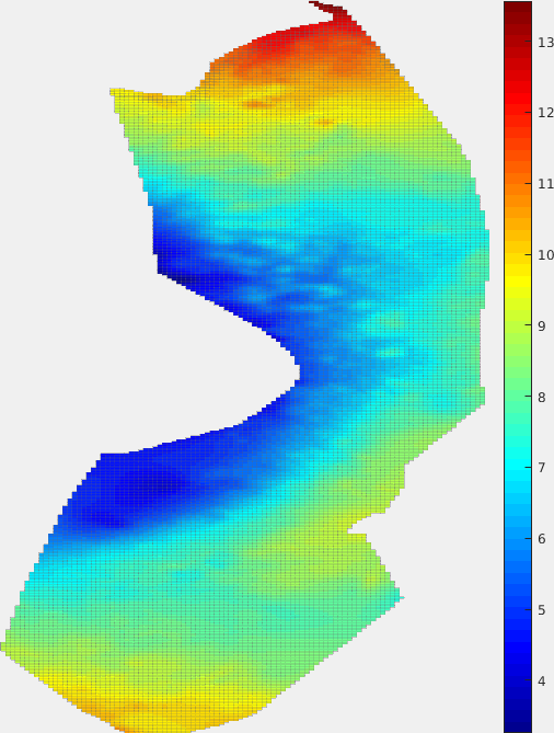
Figure 1: |
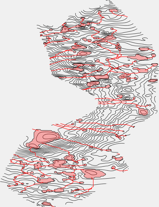
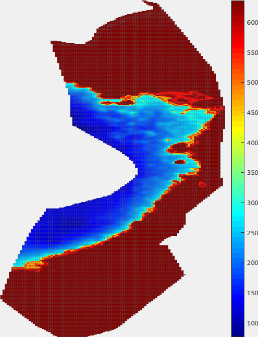
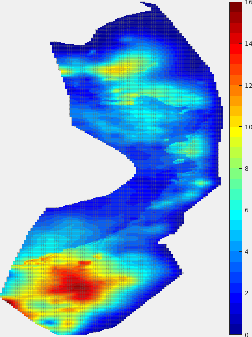
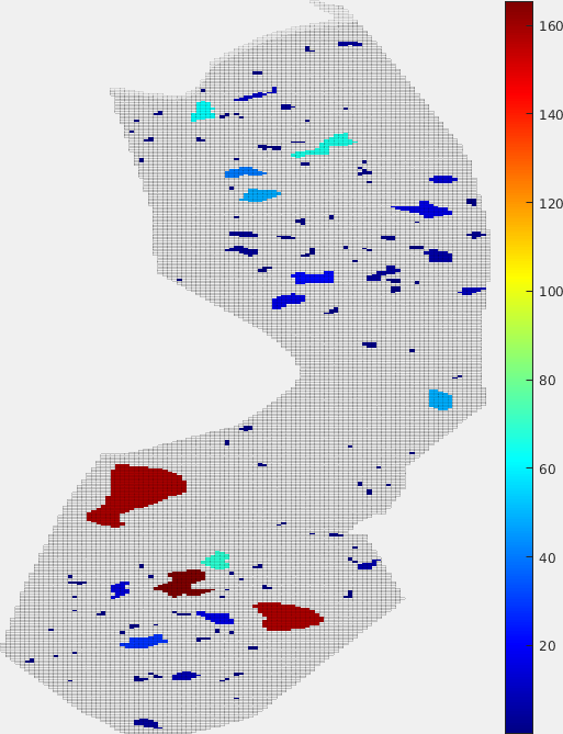
User interface
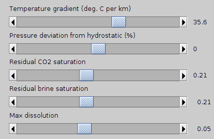
A set of radio buttons at the upper right side of the interface allows the user to specify what information should be shown along with with the geological formation in the graphical display. Below this area, a set of sliders allows the user to adjust various relevant parameters.
On the bottom right side, the current trapping capacity estimate is shown. The total figure is presented first, then its breakdown into structural, residual and dissolution trapping capacity.