Contents

Workflow example for MRST-AD

This example aims to show the complete workflow for creating, running and analyzing a simulation model. Unlike the other examples, we will create all features of the model manually to get a self-contained script without any input files required.

The model we setup is a slightly compressible two-phase oil/water model with multiple wells. The reservoir has a layered strategraphy and contains four intersecting faults. Note that this example features a simple conceptual model designed to show the workflow rather than a problem representing a realistic scenario in terms of well locations and fluid physics.

mrstModule add ad-core ad-blackoil ad-props mrst-gui
close all;

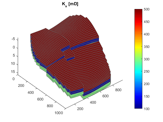
Reservoir geometry and petrophysical properties

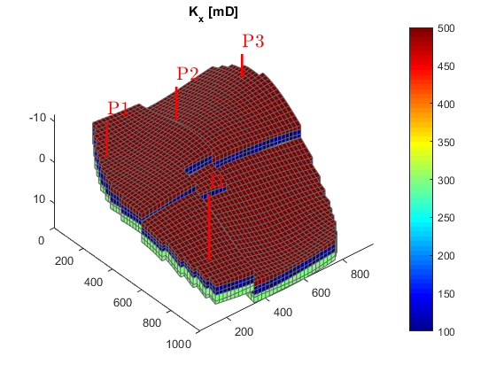
We begin by setting up the grid and rock structures. The grid is created by "makeModel3", which creates a structured model with intersecting faults. We assume a layered permeability structure with 300, 100, and 500 md in the lower, middle, and top layers. respectively.

% Define grid
grdecl = makeModel3([50, 50, 5], [1000, 1000, 5]*meter);
G = processGRDECL(grdecl);
G = computeGeometry(G);

% Set up permeability based on K-indices
[I, J, K] = gridLogicalIndices(G);

top = K < G.cartDims(3)/3;
lower = K > 2*G.cartDims(3)/3;
middle = ~(lower | top);

px = ones(G.cells.num, 1);
px(lower) = 300*milli*darcy;
px(middle) = 100*milli*darcy;
px(top) = 500*milli*darcy;

% Introduce anisotropy by setting K_x = 10*K_z.
perm = [px, px, 0.1*px];
rock = makeRock(G, perm, 0.3);

% Plot horizontal permeability and wells
figure(1); clf
plotCellData(G, rock.perm(:, 1)/(milli*darcy))
view(50, 50), axis tight
colorbar
title('K_x [mD]')

Define wells and simulation schedule

Hydrocarbon is recovered from producers, operating at fixed bottom-hole pressure and perforated throughout all layers of the model. The producers are supported by a single water injector set to inject one pore volume over 10 years (the total simulation length). We also set up a schedule consisting of 5 small control steps initially, followed by 25 larger steps. We keep the well controls fixed throughout the simulation.

simTime = 10*year;
nstep   = 25;
refine  = 5;

% Producers
pv      = poreVolume(G, rock);
injRate = 1*sum(pv)/simTime;
offset  = 10;
W = verticalWell([], G, rock, offset, offset, [],...
                'Name', 'P1', 'comp_i', [1 0], 'Val', 250*barsa, 'Type', 'bhp');
W = verticalWell(W, G, rock,  offset, floor(G.cartDims(1)/2)+3, [],...
                'Name', 'P2', 'comp_i', [1 0], 'Val', 250*barsa, 'Type', 'bhp');
W = verticalWell(W, G, rock, offset, G.cartDims(2) - offset/2, [], ...
                'Name', 'P3', 'comp_i', [1 0], 'Val', 250*barsa, 'Type', 'bhp');
% Injectors
W = verticalWell(W, G, rock, G.cartDims(1)-5, offset, 1,...
                'Name', 'I1', 'comp_i', [1 0], 'Val', injRate, 'Type', 'rate');

% Compute the timesteps
startSteps = repmat((simTime/(nstep + 1))/refine, refine, 1);
restSteps =  repmat(simTime/(nstep + 1), nstep, 1);
timesteps = [startSteps; restSteps];

% Set up the schedule containing both the wells and the timesteps
schedule = simpleSchedule(timesteps, 'W', W);

% Plot the wells
plotWell(G, W)
axis tight

Set up simulation model

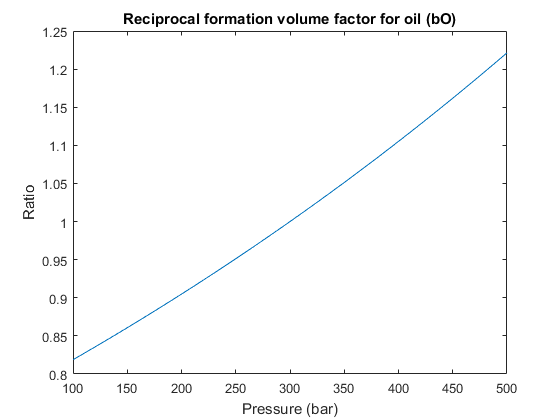
We set up a two-phase oil-water simulation model based on automatic differentiation. The resulting object is a special case of a general three-phase model and to instantiate it, we start by constructing a three-phase fluid structure with properties given for oil, water, and gas. (The gas properties will be neglected once we construct the two-phase object). Water is assumed to be incompressible, whereas oil has constant compressibility, giving a reciprocal formation volume factor of the form, . To define this relation, we set the 'bo' field of the fluid structure to be an anonymous function that calls the builtin 'exp' function with appropriate arguments. Since the fluid model is a struct containing function handles, it is simple to modify the fluid to use alternate functions. We then pass the fundamental structures (grid, rock and fluid) onto the two-phase oil/water model constructor.

% Three-phase template model
fluid = initSimpleADIFluid('mu',    [1, 5, 0]*centi*poise, ...
                           'rho',   [1000, 700, 0]*kilogram/meter^3, ...
                           'n',     [2, 2, 0]);

% Constant oil compressibility
c        = 0.001/barsa;
p_ref    = 300*barsa;
fluid.bO = @(p) exp((p - p_ref)*c);
clf
p0 = (100:10:500)*barsa;
plot(p0/barsa, fluid.bO(p0))
xlabel('Pressure (bar)')
ylabel('Ratio')
title('Reciprocal formation volume factor for oil (bO)')

% Construct reservoir model
gravity reset on
model = TwoPhaseOilWaterModel(G, rock, fluid);

Define initial state

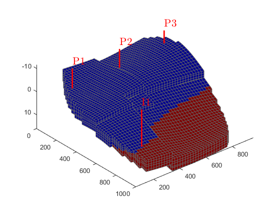
Once we have a model, we need to set up an initial state. We set up a very simple initial state; we let the bottom part of the reservoir be completely water filled, and the top completely oil filled. MRST uses water, oil, gas ordering internally, so in this case we have water in the first column and oil in the second for the saturations.

sW = ones(G.cells.num, 1);
sW(G.cells.centroids(:, 3) < 5) = 0;

sat = [sW, 1 - sW];

g = model.gravity(3);
% Compute initial pressure
p_res = p_ref + g*G.cells.centroids(:, 3).*...
   (sW.*model.fluid.rhoWS + (1 - sW).*model.fluid.rhoOS);
state0 = initResSol(G, p_res, sat);
clf
plotCellData(G, state0.s(:,1))
plotWell(G,W)
view(50, 50), axis tight

Simulate base case

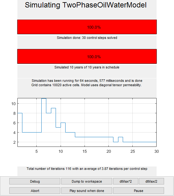
Using the schedule giving dynamic controls and time steps, the model giving the mathematical description of how to advance the solution, and the initial state of the reservoir, we can simulate the problem. Since the simulation will consume some time, we launch a progress report and a plotting tool for the well solutions (well rates and bottom-hole pressures)

fn = getPlotAfterStep(state0, model, schedule,'view',[50 50], ...
                     'field','s:1','wells',W);
[wellSols, states, report] = ...
   simulateScheduleAD(state0, model, schedule,'afterStepFn',fn);

Solving timestep 01/30:          -> 28 Days, 1 Hour, 3046.15 Seconds
Solving timestep 02/30: 28 Days, 1 Hour, 3046.15 Seconds -> 56 Days, 3 Hours, 2492.31 Seconds
Solving timestep 03/30: 56 Days, 3 Hours, 2492.31 Seconds -> 84 Days, 5 Hours, 1938.46 Seconds
...
*** Simulation complete. Solved 30 control steps in 64 Seconds, 577 Milliseconds ***

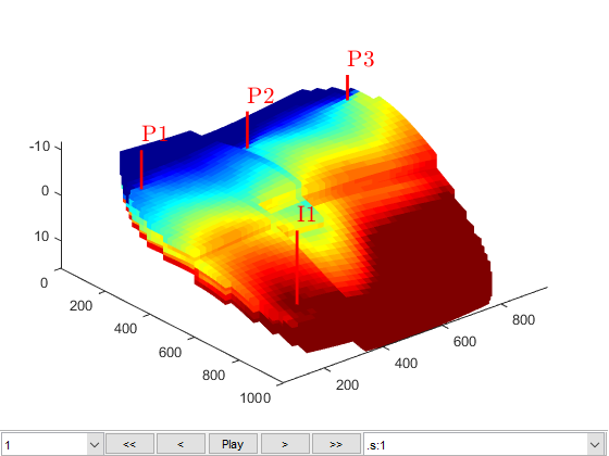
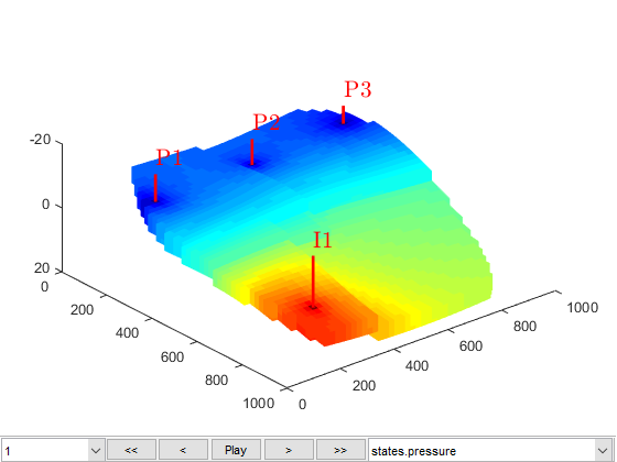
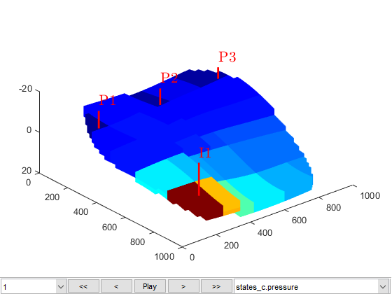
Plot reservoir states

We launch a plotting tool for the reservoir quantities (pressures and saturations, located in states).

figure(1)
plotToolbar(G, states)
view(50, 50);
plotWell(G,W);

Create an upscaled, coarser model

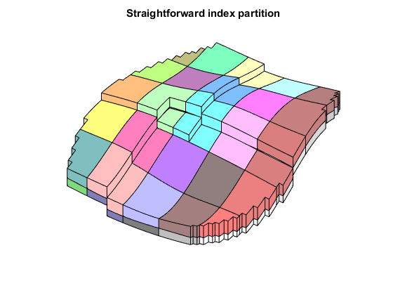
The fine scale model has approximately 10000 cells. If we want a smaller model we can easily define an upscaled model. Here we set up a simple uniform partition of approximately 50 cells based on the IJK-indices of the grid.

close([2 3]);
mrstModule add coarsegrid
cdims = [5, 5, 2];
p0 = partitionUI(G, cdims);

figp = figure;
CG = generateCoarseGrid(G,p0);
plotCellData(CG,(1:CG.cells.num)', 'EdgeColor', 'none');
plotFaces(CG,1:CG.faces.num,'EdgeColor','k','FaceColor','none');
colormap(.5*colorcube(CG.cells.num)+.5*ones(CG.cells.num,3));
axis tight off
view(125, 55)
title('Straightforward index partition');

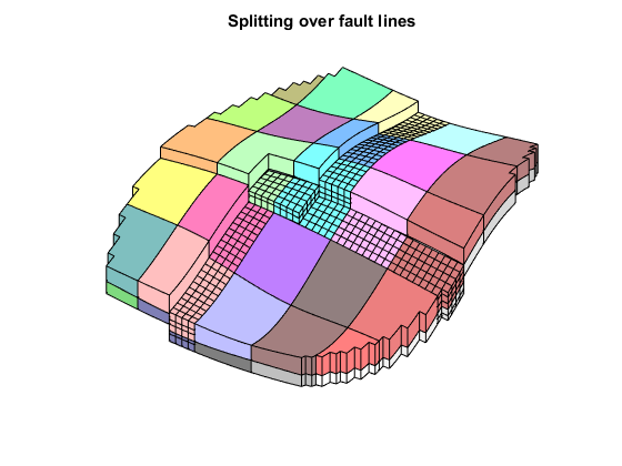
Split blocks over the faultlines

We see that several coarse blocks cross the fault lines. To get hexahedral coarse blocks, we create a grid where the faults act as barriers and apply the "processPartition" routine to split any coarse blocks intersected by faults.

Afterwards, we show the new partition and highlight blocks created due to the modification of the fault.

G_fault = makeInternalBoundary(G, find(G.faces.tag > 0));
p = processPartition(G_fault, p0);
plotGrid(G, p ~= p0, 'EdgeColor', 'w', 'FaceColor', 'none')
title('Splitting over fault lines');

Upscale the model and run the coarser problem

We can now directly upscale the model, schedule, and initial state. By default, the upscaling routine uses the simplest possible options, i.e., harmonic averaging of permeabilities. It is possible to use more advanced options, but for the purpose of this example we will use the defaults.

Once we have an upscaled model, we can again simulate the new schedule and observe that the time taken is greatly reduced. For instance, on a Intel Core i7 desktop computer, the fine model takes little under a minute to run, while the upscaled model takes 4 seconds.

clear CG; close(figp);
model_c = upscaleModelTPFA(model, p);
G_c    = model_c.G;
rock_c = model_c.rock;

schedule_c = upscaleSchedule(model_c, schedule);
state0_c = upscaleState(model_c, model, state0);

[wellSols_c, states_c] = simulateScheduleAD(state0_c, model_c, schedule_c);

Solving timestep 01/30:          -> 28 Days, 1 Hour, 3046.15 Seconds
Solving timestep 02/30: 28 Days, 1 Hour, 3046.15 Seconds -> 56 Days, 3 Hours, 2492.31 Seconds
...
*** Simulation complete. Solved 30 control steps in 3 Seconds, 270 Milliseconds ***

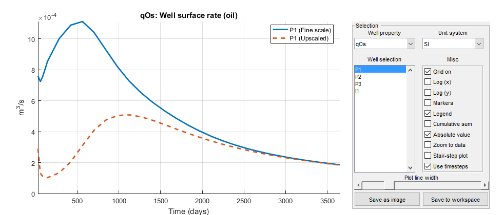
Plot the coarse results, and compare the well solutions

We plot the coarse solutions and compare the well solutions. Note that the upscaling will result in only 70 cells, which is unlikely to give good results with only simple harmonic averaging of permeabilities.

figure(2); clf
plotToolbar(G_c, states_c); plotWell(G, W)
view(50, 50);

plotWellSols({wellSols, wellSols_c}, cumsum(schedule.step.val), ...
   'DatasetNames', {'Fine scale', 'Upscaled'}, 'Field', 'qOs');

Compute flow diagnostics

As an alternative to looking at well curves, we can also look at the flow diagnostics of the models. Flow diagnostics are simple routines based on time-of-flight and tracer equations, which aim to give a qualitative understanding of reservoir dynamics. Here, we take the end-of-simulation states as a snapshot for both the fine and coarse model and compute time-of-flight and well tracers.

mrstModule add diagnostics
close(3)
D   = computeTOFandTracer(states{end},   G,   rock,   'Wells', schedule.control.W);
D_c = computeTOFandTracer(states_c{end}, G_c, rock_c, 'Wells', schedule_c.control.W);

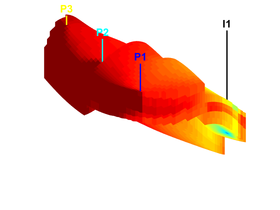
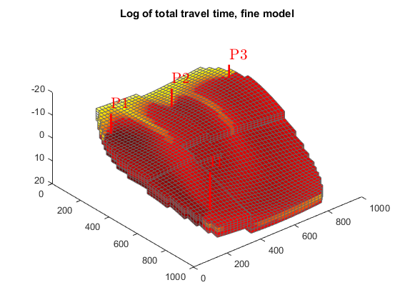
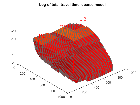
Plot total arrival times

We plot the residence time from injector to producer to separate high-flow regions, shown in dark red, from low-flow or stagnant regions, shown in yellow to white.

Since the values vary by several orders of magnitude, we plot the logarithm of the values. We also use the same color axis to ensure that the plots can be compared.

figure(1); clf, cmap=colormap;
hf = plotCellData(G, log10(sum(D.tof, 2))); plotWell(G,W)
view(50, 50); colormap(hot.^.5);
title('Log of total travel time, fine model');
c = caxis();

figure(2); clf
hc = plotCellData(G_c, log10(sum(D_c.tof, 2))); plotWell(G,W)
view(50, 50); colormap(hot.^.5);
title('Log of total travel time, coarse model');
caxis(c)

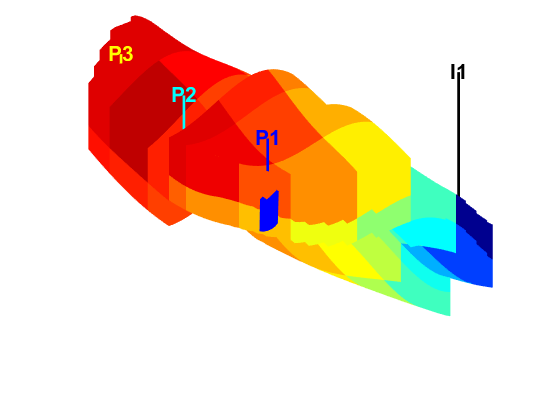
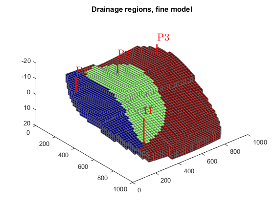
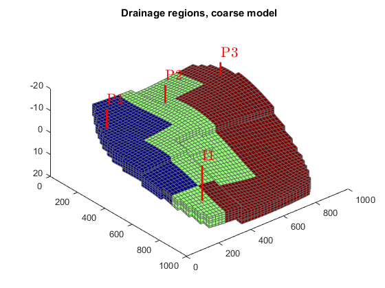
Plot tracer partitioning

We can also look at the tracer partitioning for the producers, showing the drainage regions for the different wells.

See the diagnostics module for more examples and more in-depth discussions of how flow diagnostics can be used.

figure(1); delete(hf), colormap(cmap)
plotCellData(G, D.ppart);
title('Drainage regions, fine model');

figure(2); delete(hc), colormap(cmap), caxis auto
plotCellData(G_c, D_c.ppart);
title('Drainage regions, coarse model');

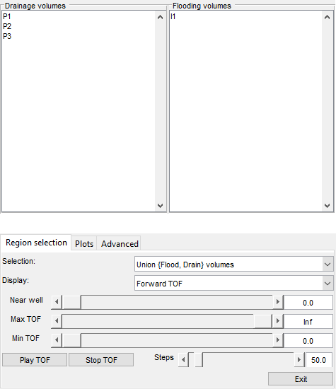
Launch interactive diagnostics tools

We can also examine the diagnostics interactively using the diagnostics viewer.

close all;
interactiveDiagnostics(G, rock, schedule.control.W, 'state', states{end}, 'computeFlux', false, 'name', 'Fine model');
interactiveDiagnostics(G_c, rock_c, schedule_c.control.W, 'state', states_c{end}, 'computeFlux', false, 'name', 'Coarse model');

New state encountered, computing diagnostics...
New state encountered, computing diagnostics...