MRSTlogo_web_banner_light_thinner_Epi.png

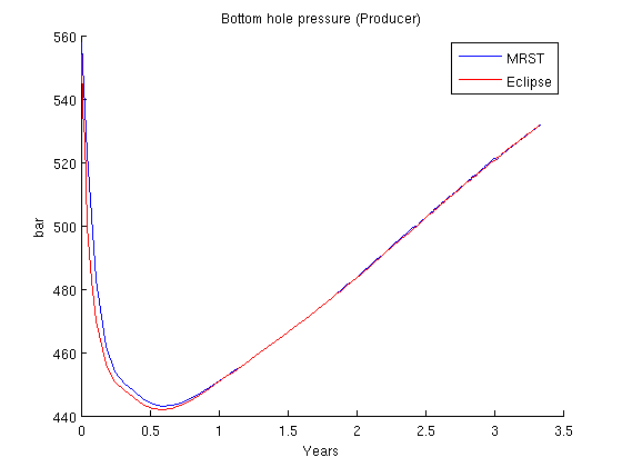
Fully implicit solve of SPE1

Contents

SPE1 case for fully implicit black oil solver

This example solves the SPE1 problem which consists of gas injection in a small ($10\times10\times3$
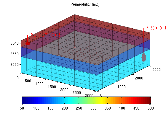
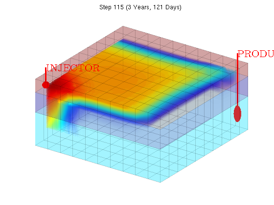
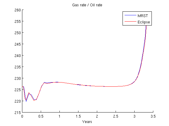
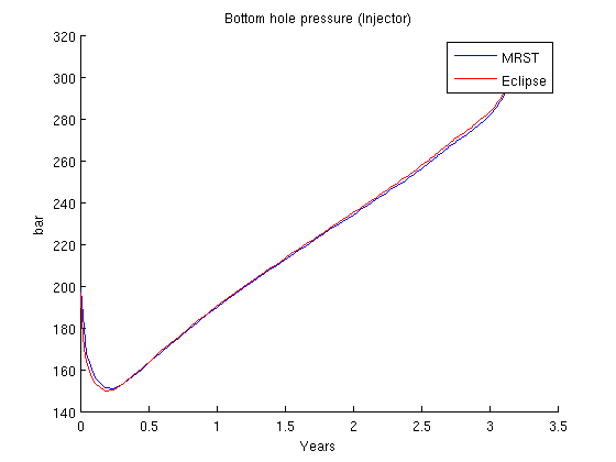
) reservoir with a single producer and injector. The problem is parsed and solved from the problem file "odeh_adi" and the result is then compared to output from a major commercial reservoir simulator (Eclipse 100).

require ad-fi deckformat

% Read and process file.
current_dir = fileparts(mfilename('fullpath'));
fn    = fullfile(current_dir, 'odeh_adi.data');

deck = readEclipseDeck(fn);

% The deck is given in field units, MRST uses metric.
deck = convertDeckUnits(deck);

G = initEclipseGrid(deck);
G = computeGeometry(G);

rock  = initEclipseRock(deck);
rock  = compressRock(rock, G.cells.indexMap);

% Create a special ADI fluid which can produce differentiated fluid
% properties.
fluid = initDeckADIFluid(deck);

% The case includes gravity
gravity on

% The initial state is provided as a binary file. The initial state
% contains a uniform mixture of water (.12) and oil (.88).
load initialState;

Plot well and permeability

The permeability consists of three layers going from high to low permeability along the z axis. The wells are completed in the upper and lower layer for the injector and producer respectively. To get a well object, we simply process the first control from the schedule.

Note that a schedule is not necessary to solve problems using the fully implicit solver: solvefiADI is capable of taking a well object directly and solving for a single time step in a manner similar to the other MRST solvers.

clf;
W = processWells(G, rock, deck.SCHEDULE.control(1));
plotCellData(G, convertTo(rock.perm(:,1), milli*darcy), 'FaceAlpha', .5, ...
            'EdgeAlpha', .3, 'EdgeColor', 'k');
plotWell(G, W);
title('Permeability (mD)')
axis tight;
view(35, 40);
colorbar('SouthOutside');

Initialize schedule and system before solving for all timesteps

We extract the schedule from the read deck and create a ADI system for our problem. The system autodetects a black oil problem and sets up default values for the various options. The only thing we change is to disable the CPR preconditioner as the problem is too small to benefit from preconditioning: The overhead required for the preconditioner is bigger than the benefits offered by a specialized solver.

During some time steps (67 and 91) the Newton iterations oscillate. The solver detects this, and dampens or relaxes the step length when this behavior is observed.

To see detailed convergence analysis during each time step, set verbose to on using

mrstVerbose on

schedule = deck.SCHEDULE;
system = initADISystem(deck, G, rock, fluid, 'cpr', false);
timer = tic;
[wellSols states iter] = runScheduleADI(state, G, rock, system, schedule);
toc(timer)

Plot the solution

We opt for a simple volume plot of the gas saturation. If opengl capability is set to software, we fall back to a simpler cell data plot. If you have problems with getting good plots you can set useVolume to false.

oglcapable = opengl('data');
useVolume = ~oglcapable.Software;

figure(1)
view(35, 40);
for i = 2:numel(states)
    [az el] = view();
    clf;

    % Plot the wells
    plotWell(G, W);
    if useVolume
        % Plot the grid as a transparent box colorized by the permeability
        plotCellData(G, convertTo(rock.perm(:,1), milli*darcy), ...
                           'FaceAlpha', .2, 'EdgeAlpha', .1, 'EdgeColor', 'k');

        % Create isosurfaces based on the gas saturation
        plotGridVolumes(G, states{i}.s(:,3), 'N', 100, 'extrudefaces', false)
    else
        plotCellData(G, states{i}.s(:,3));
    end
    time = sum(schedule.step.val(1:i-1));
    title(['Step ' num2str(i) ' (' formatTimeRange(time) ')'])
    axis tight off
    view(az, el);
    pause(.1)

end

Set up plotting

Load summary from binary file and find indices of the producer and injector.

load SPE1_smry

inj = find([wellSols{1}.sign] == 1);
prod = find([wellSols{1}.sign] == -1);

% Since there are zero values in the first step of the summary, we ignore
% the first entry to get better plot axes.
ind = 2:118;

% Put the well solution data into a format more suitable for plotting
[qWs, qOs, qGs, bhp] = wellSolToVector(wellSols);

% Get timesteps for both the reference and the MRST run
T = convertTo(cumsum(schedule.step.val), year);
Tcomp =  smry.get(':+:+:+:+', 'YEARS', ind);

Plot Producer Gas/Oil ratio

The most interesting part of the SPE1 case is the gas/oil ratio at the producer. We convert the field units and plot the dimensionless ratio. As should be apparent from the figure, the implicit solver is able to qualitatively reproduce the same outflow profile.

clf
ecl = convertFrom(smry.get('PRODUCER', 'WGOR', ind), 1000*ft^3/stb)';
mrst = qGs(:,prod)./qOs(:,prod);

hold on
plot(T, mrst)
plot(Tcomp, ecl, 'r');
legend({'MRST', 'Eclipse'})
xlabel('Years')
title('Gas rate / Oil rate')

Plot Injector Bottom Hole Pressure

The injector is rate controlled and so the bottom hole pressure is solved in the implicit loop. Plot it to verify accuracy.

clf
ecl = convertFrom(smry.get('PRODUCER', 'WBHP', ind), psia)';
mrst = bhp(:,prod);
hold on
plot(T,     convertTo(mrst, barsa))
plot(Tcomp, convertTo(ecl, barsa), 'r');
legend({'MRST', 'Eclipse'})
xlabel('Years')
ylabel('bar')
title('Bottom hole pressure (Producer)')

Plot Injector Bottom Hole Pressure

clf
ecl = convertFrom(smry.get('INJECTOR', 'WBHP', ind), psia)';
mrst = bhp(:,inj);
hold on
plot(T,     convertTo(mrst, barsa))
plot(Tcomp, convertTo(ecl, barsa), 'r');
legend({'MRST', 'Eclipse'})
xlabel('Years')
ylabel('bar')
title('Bottom hole pressure (Producer)')

Published November 23, 2016