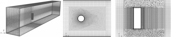
Background
Structure and design of fish cages can be improved by the knowledge of the flow pattern around and inside the net cages. To address this problem, commercially available computational fluid dynamics (CFD) software is used to analyze this problem by calculating the drag and the flow velocity distribution around cylinders with different porosities. Aquaculture cages are very large structures that consist mainly of netting, which can be approximated by small cylinders connected at knots. But due to the large number of these cylinders (millions for a single salmon farming cage), it is computationally expensive to model the exact geometry. Biofouling is another factor which is of particular interest as fouled nets (lower porosity) can significantly reduce flow of well-oxygenated water reaching the fish during normal rearing conditions. Therefore the numerical approach used to simulate the flow through and around the net cage is to consider it as a circular cylinder with a porous jump boundary. Drag coefficient and flow pattern are compared with available experimental data. Vertical cylinders are used for this study. Different porosities have been used for the simulations as for the experiments in order to simulate the impact of the fouling on the load of the net structures and the flushing of the cage. The results show that a porous jump with a pressure drop proportional to velocity squared has the best agreement with measured data.

Methods
Numerical simulations have been performed for towing tested in water channel which are vertical solid cylinder and 20% ~ 90% porosity cylinders at 0.05 m/s inlet velocity. In this study, FLUENT a commercial CFD program is used for the simulation; it is based on the Finite Volume Method. The fluid dynamics for Analysis of fish cages with porous boundary condition basically consists with continuity equation and momentum conservation equations. Incompressible flow is used for these steady state simulations and turbulence is modelled by using the realizable k-ε model. The SIMPLE (Semi-Implicit Method for Pressure-Linked Equations) algorithm was used for pressure–velocity coupling. A first order upwind scheme is used for discretization. Maximum residual tolerance was set under the 1×10E-6. Figure 1 shows grid system for solid and porous cylinder. A mixed (hexahedral and tetrahedral) cell model was used for numerical simulation, and was chosen by a mesh independent test. In order to simulate the porosity of a net cage the porous jump boundary condition available in the FLUENT package was used introduced : Porous boundary this condition can be used for modeling a wide variety of engineering applications, including flows through packed beds, filters, perforated plates, flow distributors and tube banks. It is generally desirable to determine the pressure drop across the porous area and to predict the flow field in order to optimize a given design. Porous jump conditions are used to model a thin membrane that has known velocity (pressure-drop) characteristics. This simpler model has been used instead of the full porous media model also available, because of its robustness and better convergence.

Figure 1 3D view of the complete grid (left), sectional view in XY plane (middle) and sectional view in XZ plane (right).

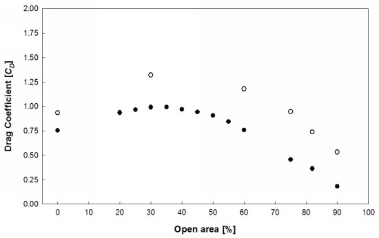
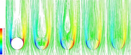
Suitable for CFD simulation with porous boundary condition investigated apply to flow analysis on fish cages. The drag coefficient on the model were calculated as
 ,
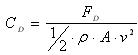
where   is the drag coefficient,   is the drag force,  is the density of fluid   is the projected area of the cylinder and  is the inflow velocity. Figure 2 shows drag coefficient comparison of solid and porous cylinder at Re=5000. Drag force from the experiment of Gansel et al.(2008) with time averaged has been calculated on 20cm. Random events usually happen on small time scales than periodic events like vortex shedding. It is therefore necessary to use time series for the time averages calculation that are long enough to include several cycles of periodic events. And the towing arrangement consists of one cylinder attached to a circular end-plate. The diameter of the plate is 3D. According to this reason, the experiment drag coefficient of the solid cylinder for Re=5000 shows higher drag coefficient than the simulation results. However the trend of drag coefficient shows a good agreement with regular intervals between experiment and simulation. The drag coefficient decreases with the increasing open area (%) of the porous models after 30 and 35% open area. Meanwhile 20 and 25% open area cylinder indicate lower drag coefficient than 30 and 35% open area cylinder. This is interesting results due to describe a parabola as increase open area. Noymer et al. (1998) used the Darcy model to describe the flow through the porous cylinder. A peak zone in the drag ratio was observed at Re=100 and Re=1000. Present simulation results are in very similar pattern with them as increase open area (%). The streamlines as increase open area is presented in Figure 3 for Re=5000. For a solid cylinder, the vorticity diffuses from the surface into the external flow field, whereas, for all of porous cylinder vorticity diffuses into both the external and internal flow fields. At 20% open cylinder, a stream entering the porous cylinder generate recirculation zone at the inside of the cylinder due to the recirculation set up by the external field at the rear end. At 25% open cylinder, a stream can not pass right through the porous cylinder, because of the recirculation still exist by the external field at the 1 diameter downstream from the centre of the cylinder. Hence the streamline pass along the cylinder and then bypasses the recirculation zone. 30% and 40% open cylinder can not see the recirculation zone at the inside and rear of cylinder. Less bypass flow and the increased velocity of the fluid at the interface may leads to increased drag coefficient for 30% open cylinder. The angle of flow separation from the porous cylinders is 124^o for 20% open cylinder, 118^o for 30% open cylinder and 127^o for 40% open cylinder. The separation angle is measured from the front stagnation point. It is corroborative facts from the pick zone in the drag coefficient that the separation point shifts towards the front and rear stagnation point with 30% open area cylinder as the centre. The porous cylinder allows a finite amount of fluid to pass through with a non-zero velocity at the interface. With increasing open area after 30% the velocity of the fluid at the interface increases. This velocity has the effect of reducing the relative importance of the inertial forces in the external field.

Figure 2 Drag coefficient comparison with experiment and simulation for 0% ~ 90% open cylinder at Re=5000. ○: Gansel et al.(2008) experiment; ●: present simulation.

Figure 3 Streamlines for the flow through the cylinder rendered by contours of the z-vorticity in the z/D=1.5 at Re=5000 (a) 0% open cylinder; (b) 20% open cylinder; (c) 25% open cylinder; (d) 30% open cylinder and (e) 40% open cylinder.

        a)                               b)                               c)                                  d)                               e)