Two-Dimensional Riemann Problems for Ideal Gas Dynamics
The compressible
Euler equations describing the flow of an ideal gas is a particular example
of hyperbolic systems. Since the mathematical structure of the solution to the
Euler equations is well-understood, this system serves as the main benchmark
for testing new numerical methods developed for fluid dynamics
problems with a similar mathematical character.
The Riemann problem is the simplest possible initial value problem
for hyperbolic systems. In one spatial dimension, the
Riemann (or shock-tube) problem is composed of two uniform states in the
infinite domain separated by a discontinuity at the origin. For the Euler
equations the
exact solution of the Riemann problem is well-known, self-similar, and
consists of a combination of three wave types: shocks (S), rarefaction waves
(R), and contact discontiunitites (R). Apart from being an important
testbench, the Riemann problem is a basic building block for a large class of
modern numerical methods, called upwind or Godunov
schemes.
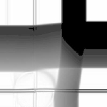
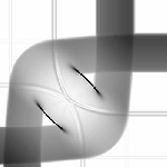
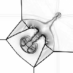
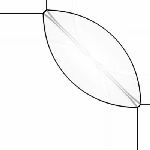
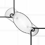
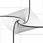
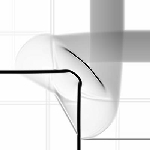
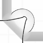
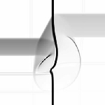
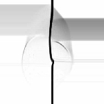
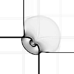
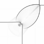
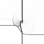
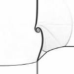
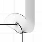
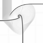
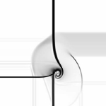
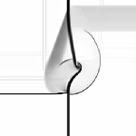
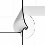
In two-spatial dimensions, the Riemann problems consists of four uniform
states, one in each quadrant. Compared with the relatively simple wave
patterns in the 1-D case, the 2-D case gives rise to quite complicated wave
patterns. These patterns can be characterised as 19 different configurations
(see Schulz-Rinne, Collins and Glaz, SIAM J. Sci. Comp., Vol 14, No. 6, 1993),
as shown in the images (and movies) below. The solutions are computed using a
second-order,
staggered, nonoscillatory, central difference scheme. The same 19 cases
have been studied previously by Kurganov
and Tadmor using related central difference schemes. The solutions are
plotted as emulated Schlieren images by
depicting the norm of the density gradient in a nonlinear graymap. This
visualisation technique is particulary useful for depicting gradients in the
density, but is also excellent for enhancing small-scale variances, for
instance, the small numerical artifacts seen in several of the images below
(pairs of horisontal and vertical lines).
 |
 |
 |
 |
 |
| Configuration 1 |
Configuration 2 |
Configuration 3 |
Configuration 4 |
Configuration 5 |
|
 |
 |
 |
 |
 |
| Configuration 6 |
Configuration 7 |
Configuration 8 |
Configuration 9 |
Configuration 10 |
|
 |
 |
 |
 |
 |
| Configuration 11 |
Configuration 12 |
Configuration 13 |
Configuration 14 |
Configuration 15 |
|
 |
 |
 |
 |
| Configuration 16 |
Configuration 17 |
Configuration 18 |
Configuration 19 |
Contact: Knut-Andreas
Lie ( Knut-Andreas.Lie@math.sintef.no)
Last updated: February 2002.