This example demonstrates how to perform a single-phase upscaling of the absolute permeability for a 2D Cartesian model. The routines we use are also applicable in 3D.

Contents

Load the required modules

try
   require upscaling coarsegrid
catch %#ok<CTCH>
   mrstModule add upscaling coarsegrid
end
verbose = true;

Define fine-scale model and coarse grid

We consider two different grids: a fine scale grid that represents the original model and a coarse-scale grid that represents the upscaled model in a way that is independent of the original fine-scale model. For the fine-scale model we define a lognormal permeability field.

cellDims  = [15 15 1];
G         = cartGrid(cellDims, cellDims);
G         = computeGeometry(G);
K         = exp( 5*gaussianField(cellDims, [-1 1], [7 7 1]) + 1);
rock.perm = convertFrom(K(:), milli()*darcy());

% The coarse grid
upscaled  = [5 5 1];
G_ups     = cartGrid(upscaled, cellDims);
G_ups     = computeGeometry(G_ups);

Compute upscaled permeability

To compute the upscaled permeability, we need to define a coarse-grid structure that describes how the coarse grid relates to the fine grid. In our case, this is simple: the coarse grid is uniform partition of the fine grid.

p  = partitionUI(G, upscaled);
p  = processPartition  (G, p, 'Verbose', verbose);
CG = generateCoarseGrid(G, p, 'Verbose', verbose);

rockUps.perm = upscalePerm(G, CG, rock, 'Verbose', verbose);

Elapsed time is 0.079428 seconds.
Computing upscaled permeabilities... Elapsed time is 0.274742 seconds.

Plot permeabilities

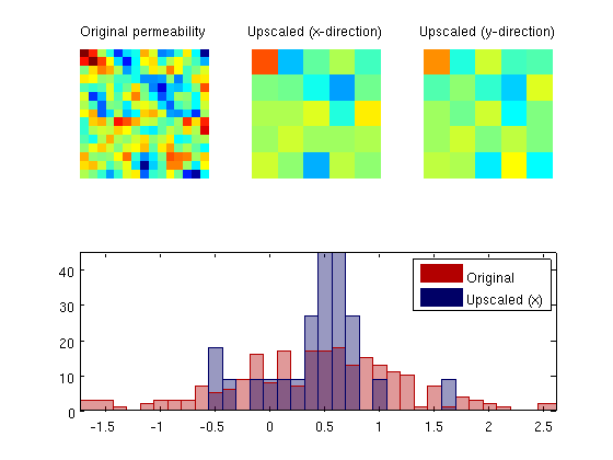
Whereas the fine-scale permeability field is isotropic, the upscaled permeability field is anisotropic and we therefore plot both the components in both directions. In addition, we present a histogram of the original permeability and the upscaled permeability projected back onto the fine grid to more clearly show how upscaling reduces the span and tends to cluster values around the median of the fine-scale distribution.

clf
subplot(2,3,1)
plotCellData(G, log10(rock.perm));axis equal tight off
coaxis = caxis; title('Original permeability')

subplot(2,3,2)
plotCellData(G_ups, log10(rockUps.perm(:,1)));  axis equal tight off
title('Upscaled (x-direction)'); caxis(coaxis)

subplot(2,3,3)
plotCellData(G_ups,  log10(rockUps.perm(:,2)));  axis equal tight off
title('Upscaled (y-direction)'); caxis(coaxis)

subplot(2,3,4:6)
bins = -1.5:0.125:2.5;
hist(log10(rock.perm(:))-log10(milli*darcy),bins);
hold on;
hist(log10(rockUps.perm(p(:),1))-log10(milli*darcy),bins);
hold off
h=get(gca,'Children');
set(h(1),'EdgeColor',[0 0 0.4],'FaceColor',[0 0 .4],'FaceAlpha',.4);
set(h(2),'EdgeColor',[0.7 0 0],'FaceColor',[.7 0 0],'FaceAlpha',.4);
axis tight
legend('Original','Upscaled (x)');

Compare models

To compare the models, we set up a simple case with a unit pressure drop from south to north and compare the normal velocities on the outflow boundary to the north. Fluid parameters are typical for water.

fluid     = initSingleFluid('mu' ,    1*centi*poise     , ...
                            'rho', 1014*kilogram/meter^3);
% Fine-scale problem
bc        = pside([], G, 'North', 0);
faces     = bc.face;
bc        = pside(bc, G, 'South',  1*barsa());
T         = computeTrans(G, rock);
xRef      = incompTPFA(initResSol(G,0), G, T, fluid, 'bc', bc);

% Coarse-scale problem
bc_ups    = pside([], G_ups, 'North', 0);
faces_ups = bc_ups.face;
bc_ups    = pside(bc_ups, G_ups, 'South', 1*barsa());
T_ups     = computeTrans(G_ups, rockUps);
xUps      = incompTPFA(initResSol(G_ups,0), G_ups, T_ups, fluid, 'bc', bc_ups);

Compare outflow

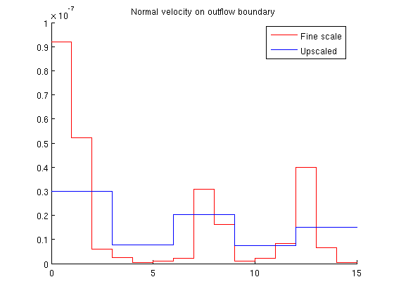
The smoothing effect of the upscaling procedure is apparent. Whereas the total outflow is very close in the two models, we see that there is significant variation in the fine-scale model that is not captured by the coarse-scale model.

flux1 = sum(xRef.flux(faces));
flux2 = sum(xUps.flux(faces_ups));
disp(['Sum outflux on fine scale   : ', num2str(flux1)]);
disp(['Sum outflux on coarse scale : ', num2str(flux2)]);

flux1_face = xRef.flux(faces)    ./G.faces.areas(faces);
flux2_face = xUps.flux(faces_ups)./G_ups.faces.areas(faces_ups);
clf; hold on
x = G.faces.centroids(faces,1); dx = diff(x);
stairs([x-.5*dx(1); x(end)+.5*dx(end)], flux1_face([1:end end]), 'r-')
x = G_ups.faces.centroids(faces_ups,1); dx = diff(x);
stairs([x-.5*dx(1); x(end)+.5*dx(end)], flux2_face([1:end end]), 'b-')
hold off
title('Normal velocity on outflow boundary')
legend({'Fine scale', 'Upscaled'},'Location','best')

Sum outflux on fine scale   : 2.6179e-07
Sum outflux on coarse scale : 2.4211e-07

Published with MATLAB® 7.9