MRSTlogo_web_banner_light_thinner_Epi.png

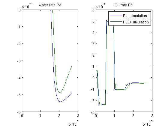
Proper Orthogonal Decomposition Example

Reservoir simulation using Proper Orthogonal Decomposition (POD)

This example demonstrates the use of model reduction when solving a given system for many small variations of the same schedule. The example is meant to illustrate the principles, not best practice for real cases.

Contents

Setup

Load required modules and set random stream

require deckformat ad-fi

s = RandStream('mcg16807','Seed',0);
RandStream.setGlobalStream(s);

% We set up a training simulation and an actual problem. The training
% simulation has the same well and grid setupm, but the BHP of the
% producers varies in the different simulations.

current_dir = fileparts(mfilename('fullpath'));
fn    = fullfile(current_dir, 'training.data');

deck_training = readEclipseDeck(fn);
deck_training = convertDeckUnits(deck_training);


fn   = fullfile(current_dir, 'problem.data');
deck_problem = readEclipseDeck(fn);
deck_problem = convertDeckUnits(deck_problem);

% The grid is common for both simulations
grd = deck_training.GRID;

G = initEclipseGrid(deck_training);
G = computeGeometry(G);

% rock - heterogenous field
poro = gaussianField(G.cartDims, [.4 .8], [11 3 3], 2.5);

K = poro.^3.*(1e-5)^2./(0.81*72*(1-poro).^2);
rock.perm    = K(:);
rock.poro = poro(:);

% fluid
fluid = initDeckADIFluid(deck_training);

gravity off

state.pressure = 1.5e7*ones(G.cells.num, 1);
state.s        = ones(G.cells.num,1)*[0, 1];


schedule_training = deck_training.SCHEDULE;
schedule_problem  = deck_problem.SCHEDULE;

Solve full system for various parameters to create snapshot ensamble

systemOW =      initADISystem({'Oil', 'Water'}, G, rock, fluid);
[wsol, states] = runScheduleADI(state, G, rock, systemOW, schedule_training);

Plot the simulation for all timesteps

The dominant producer switches between each control. This is obviously not a good schedule for oil production, but it gives a highly dynamic flow pattern.

figure(1);
for i = 1:numel(states)
    clf;
    subplot(2,1,1)
    plotCellData(G, states{i}.pressure)
    title('Pressure')
    subplot(2,1,2)
    plotCellData(G, states{i}.s(:,1))
    title('Water saturation')
    pause(.1);
end

Create basis for proper orthogonal decomposition

When doing model reduction, parts of the model can be reduced based on the assumption that the eigenspace of the simulation is similar to the eigenspace of the history we are using to construct the basis. As the pressure solution is costly and in general very smooth, we opt to reduce the pressure variable. This is done by a singular value decomposition and then using the largest eigenvalues to find the eigenvalues which capture the most essential patterns of pressure.

We reduce the number of pressure variables from 900 to 25. Saturation is more difficult to reduce accurately, requiring a magnitude more variables and clustering of eigenvectors. This example defaults to no clustering as the implementation of clustering depends on an external package YAEL (https://gforge.inria.fr/)

ns = nan;
np = 25;

basis_no_cluster = basisOW(states,...
                'energyfraction_pressure',  1,...
                'energyfraction_saturation',1,...
                 'maxno_pressure',          np,...
                 'maxno_saturation',        ns...
                 );

basis = basis_no_cluster;

% Copy system
systemOW_basis = systemOW;

% Add basis, set max iterations as the solution will not generally converge
% when approximated by another eigenspace.

systemOW_basis.podbasis = basis;
systemOW_basis.nonlinear.maxIterations = 6;
25 of 47 eigenvalues included
Including saturation equations in full!

Run another schedule both using pod and a full solution

The schedule is the same in terms of well setup, grid, porosity/permeability as well as the general flow pattern, but the rates have been changed. This is typical of an optimization loop: Several similar configurations which share many properties will be solved, either manually by a reservoir engineer or by a automated optimization program.

In general, a model reduction will not converge fully. We simply limit the number of iterations. A more sophisticated approach would involve setting the convergence limits based on the amount of reduction done.

timer = tic;
[wsol_full, states_full] = runScheduleADI(state, G, rock, systemOW, schedule_problem);
tfull = toc(timer);

warning('off', 'newt:maxit')
timer = tic;
[wsol_pod, states_pod]   = runScheduleADI(state, G, rock, systemOW_basis, schedule_problem);
tpod = toc(timer);
warning('on', 'newt:maxit')

Plot and compare the solutions

v = [0, 90];
figure(1);
for i = 1:numel(states_pod)
    clf;
    subplot(2,2,1)
    plotCellData(G, states_full{i}.pressure)
    title('Pressure, full solve');
    axis tight;
    cp = caxis();
    subplot(2,2,2)
    plotCellData(G, states_full{i}.s(:,1))
    title('Water saturation, full solve');
    axis tight;
    colorbar();
    cs = caxis();
    view(v);

    subplot(2,2,3)
    plotCellData(G, states_pod{i}.pressure)
    title('Pressure, reduced solve');
    axis tight;
    caxis(cp);
    subplot(2,2,4)
    plotCellData(G, states_pod{i}.s(:,1))
    title('Water saturation, reduced solve');

    caxis(cs);
    axis tight;
    err = @(x, y) abs(x-y)/x;

    colorbar();
    view(v);
    pause(.1);
end

Plot the well rates

The oil rate is in general close to the reference. The water cuts show a similar error. Note that this example was made to produce interesting flow patterns, not realistic production (oil is being injected during certain time steps).

In terms of time used, these examples are so small that the overhead of setting up the linear systems is large compared to the cost of solving the actual systems. As such, the model

time = cumsum(schedule_problem.step.val) ;
[qWsp, qOsp, qGsp, bhpp] = wellSolToVector(wsol_pod);
[qWsf, qOsf, qGsf, bhpf] = wellSolToVector(wsol_full);
for i = 2:5
    figure(i);
    clf;
    subplot(1,2,1)
    plot(time, -[qWsf(:,i) , qWsp(:,i)])
    title(['Water rate ' wsol_full{1}(i).name])
    subplot(1,2,2)
    plot(time, -[qOsf(:,i) , qOsp(:,i)])
    title(['Oil rate ' wsol_full{1}(i).name])
    legend({'Full simulation', 'POD simulation'})
end

Published December 20, 2012